Running and Combining Multiple MCMC Chains

Motivation

Mixing of an MCMC sampler is a perennial concern for complex Bayesian models. BART and BCF are no exception. One common way to address such concerns is to run multiple independent “chains” of an MCMC sampler, so that if each chain gets stuck in a different region of the posterior, their combined samples attain better coverage of the full posterior.

This idea works with the classic “root-initialized” MCMC sampler of Chipman et al. (2010), but a key insight of He and Hahn (2023) and Krantsevich et al. (2023) is that the GFR algorithm may be used to warm-start initialize multiple chains of the BART / BCF MCMC sampler.

Operationally, the above two approaches have the same implementation (setting num_gfr > 0 if warm-start initialization is desired), so this vignette will demonstrate how to run a multi-chain sampler sequentially or in parallel.

Setup

R

library(stochtree)
library(ggplot2)
library(coda)
library(bayesplot)
library(foreach)
library(doParallel)

Python

import numpy as np
import matplotlib.pyplot as plt
import arviz as az
from stochtree import BARTModel

rng = np.random.default_rng(1111)

Demo 1: Supervised Learning

Data Simulation

Simulate a simple partitioned linear model.

R

# Generate the data
set.seed(1111)
n <- 500
p_x <- 10
p_w <- 1
snr <- 3
X <- matrix(runif(n * p_x), ncol = p_x)
leaf_basis <- matrix(runif(n * p_w), ncol = p_w)
f_XW <- (((0 <= X[, 1]) & (0.25 > X[, 1])) *
  (-7.5 * leaf_basis[, 1]) +
  ((0.25 <= X[, 1]) & (0.5 > X[, 1])) * (-2.5 * leaf_basis[, 1]) +
  ((0.5 <= X[, 1]) & (0.75 > X[, 1])) * (2.5 * leaf_basis[, 1]) +
  ((0.75 <= X[, 1]) & (1 > X[, 1])) * (7.5 * leaf_basis[, 1]))
noise_sd <- sd(f_XW) / snr
y <- f_XW + rnorm(n, 0, 1) * noise_sd

# Split data into test and train sets
test_set_pct <- 0.2
n_test <- round(test_set_pct * n)
n_train <- n - n_test
test_inds <- sort(sample(1:n, n_test, replace = FALSE))
train_inds <- (1:n)[!((1:n) %in% test_inds)]
X_test <- X[test_inds, ]
X_train <- X[train_inds, ]
leaf_basis_test <- leaf_basis[test_inds, ]
leaf_basis_train <- leaf_basis[train_inds, ]
y_test <- y[test_inds]
y_train <- y[train_inds]

Python

n, p_x, p_w, snr = 500, 10, 1, 3
X = rng.uniform(size=(n, p_x))
leaf_basis = rng.uniform(size=(n, p_w))
f_XW = (((0 <= X[:, 0]) & (0.25 > X[:, 0])) * (-7.5 * leaf_basis[:, 0]) +
        ((0.25 <= X[:, 0]) & (0.5 > X[:, 0]))  * (-2.5 * leaf_basis[:, 0]) +
        ((0.5 <= X[:, 0]) & (0.75 > X[:, 0]))  * (2.5  * leaf_basis[:, 0]) +
        ((0.75 <= X[:, 0]) & (1 > X[:, 0]))     * (7.5  * leaf_basis[:, 0]))
noise_sd = np.std(f_XW) / snr
y = f_XW + rng.normal(0, noise_sd, size=n)

test_set_pct = 0.2
n_test = round(test_set_pct * n)
test_inds  = rng.choice(n, n_test, replace=False)
train_inds = np.setdiff1d(np.arange(n), test_inds)
X_test,          X_train          = X[test_inds],          X[train_inds]
leaf_basis_test, leaf_basis_train = leaf_basis[test_inds], leaf_basis[train_inds]
y_test,          y_train          = y[test_inds],          y[train_inds]

Sampling Multiple Chains Sequentially from Scratch

The simplest way to sample multiple chains of a stochtree model is to do so “sequentially,” that is, after chain 1 is sampled, chain 2 is sampled from a different starting state, and similarly for each of the requested chains. This is supported internally in both the bart() and bcf() functions, with the num_chains parameter in the general_params list.

Define some high-level parameters, including number of chains to run and number of samples per chain. Here we run 4 independent chains with 2000 MCMC iterations, each of which is burned in for 1000 iterations.

R

num_chains <- 4
num_gfr <- 0
num_burnin <- 1000
num_mcmc <- 2000

Python

num_chains = 4
num_gfr    = 0
num_burnin = 1000
num_mcmc   = 2000

Run the sampler.

R

bart_model <- stochtree::bart(
  X_train = X_train,
  leaf_basis_train = leaf_basis_train,
  y_train = y_train,
  num_gfr = num_gfr,
  num_burnin = num_burnin,
  num_mcmc = num_mcmc,
  general_params = list(num_chains = num_chains)
)

Python

bart_model = BARTModel()
bart_model.sample(
    X_train=X_train, leaf_basis_train=leaf_basis_train, y_train=y_train,
    num_gfr=num_gfr, num_burnin=num_burnin, num_mcmc=num_mcmc,
    general_params={"num_threads": 1, "num_chains": num_chains},
)

BARTModel run with mean forest, global error variance model, and mean forest leaf scale model
Outcome was modeled as gaussian with a leaf regression prior with 1 bases for the mean forest
Outcome was standardized
The sampler was run for 0 GFR iterations, with 4 chains of 1000 burn-in iterations and 2000 MCMC iterations, retaining every iteration (i.e. no thinning)

Now we have a model with num_chains * num_mcmc samples stored internally. These samples are arranged sequentially, with the first num_mcmc samples corresponding to chain 1, the next num_mcmc samples to chain 2, etc.

Since each chain is a set of samples of the same model, we can analyze the samples collectively, for example, by looking at out-of-sample predictions.

R

y_hat_test <- predict(
  bart_model,
  X = X_test,
  leaf_basis = leaf_basis_test,
  type = "mean",
  terms = "y_hat"
)
plot(y_hat_test, y_test, xlab = "Predicted", ylab = "Actual")
abline(0, 1, col = "red", lty = 3, lwd = 3)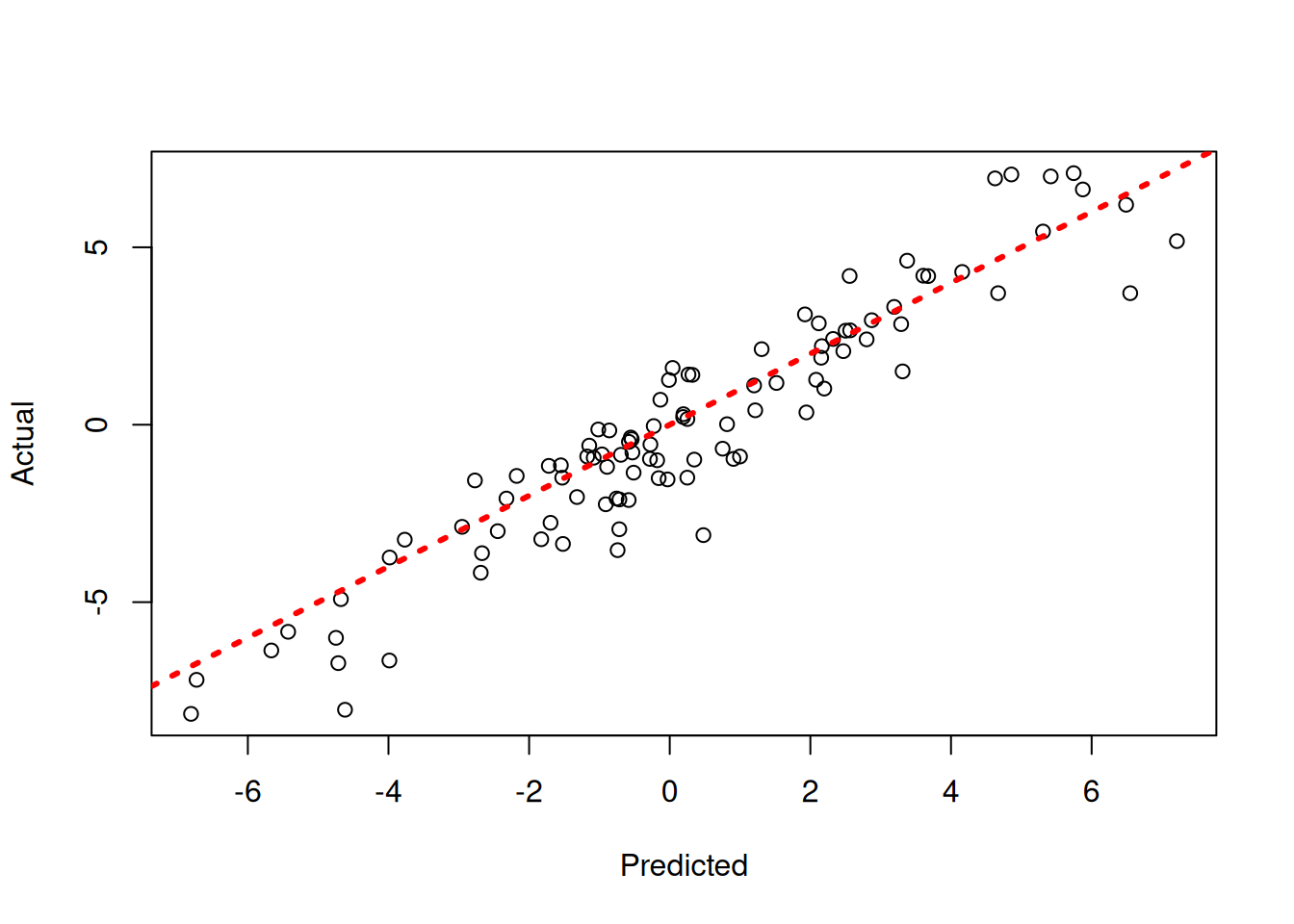

Python

y_hat_test = bart_model.predict(
    X=X_test, leaf_basis=leaf_basis_test, type="mean", terms="y_hat"
)
lo, hi = min(y_hat_test.min(), y_test.min()), max(y_hat_test.max(), y_test.max())
plt.scatter(y_hat_test, y_test, alpha=0.5)
plt.plot([lo, hi], [lo, hi], color="red", linestyle="dashed", linewidth=2)
plt.xlabel("Predicted"); plt.ylabel("Actual")
plt.show()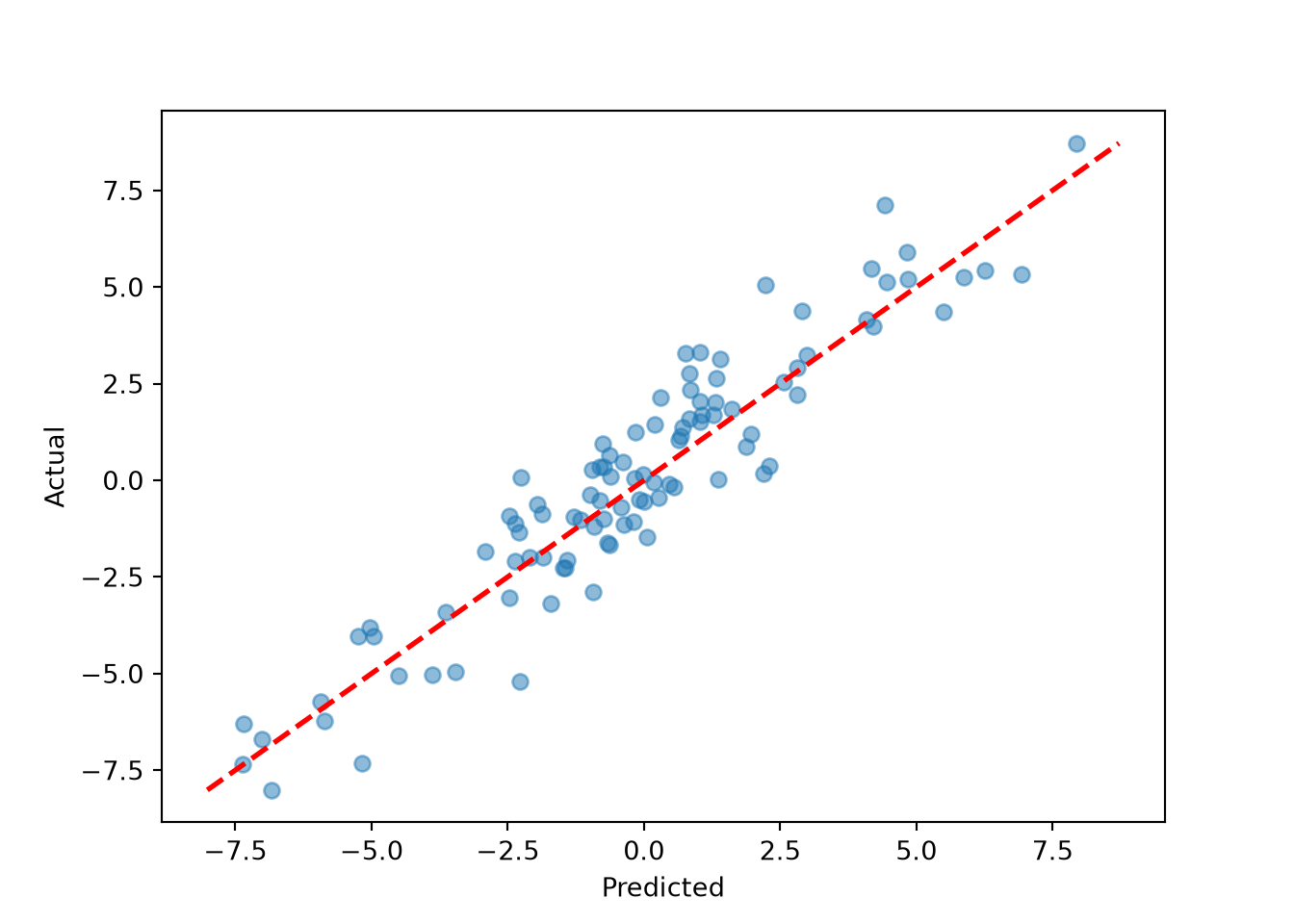

Now, suppose we want to analyze each of the chains separately to assess mixing / convergence. We can construct an mcmc.list in the coda package to perform various diagnostics.

R

sigma2_coda_list <- coda::as.mcmc.list(lapply(
  1:num_chains,
  function(chain_idx) {
    offset <- (chain_idx - 1) * num_mcmc
    inds_start <- offset + 1
    inds_end <- offset + num_mcmc
    coda::mcmc(extractParameter(bart_model, "sigma2_global")[inds_start:inds_end])
  }
))
traceplot(sigma2_coda_list, ylab = expression(sigma^2))
abline(h = noise_sd^2, col = "black", lty = 3, lwd = 3)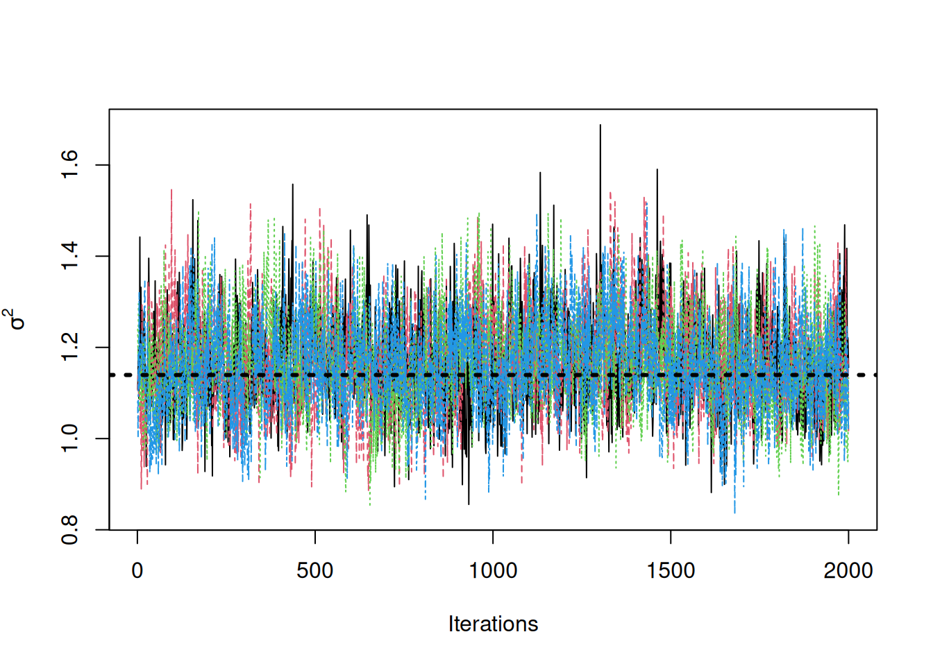

acf <- autocorr.diag(sigma2_coda_list)
ess <- effectiveSize(sigma2_coda_list)
rhat <- gelman.diag(sigma2_coda_list, autoburnin = F)
cat(paste0(
  "Average autocorrelation across chains:\n",
  paste0(paste0(rownames(acf), ": ", round(acf, 3)), collapse = ", "),
  "\nTotal effective sample size across chains: ",
  paste0(round(ess, 1), collapse = ", "),
  "\n'R-hat' potential scale reduction factor of Gelman and Rubin (1992)): ",
  paste0(round(rhat$psrf[, 1], 3), collapse = ", ")
))

Average autocorrelation across chains:
Lag 0: 1, Lag 1: 0.385, Lag 5: 0.155, Lag 10: 0.119, Lag 50: 0.029
Total effective sample size across chains: 1313.8
'R-hat' potential scale reduction factor of Gelman and Rubin (1992)): 1.001

Python

# Reshape flat sigma2 samples into (num_chains, num_mcmc) for per-chain diagnostics
# az.from_dict requires nested dict: {"posterior": {"var": array(chains, draws)}}
idata = az.from_dict({"posterior": {"sigma2": bart_model.global_var_samples.reshape(num_chains, num_mcmc)}})

<string>:3: DeprecationWarning: `BARTModel.global_var_samples` is deprecated and will be removed in a future release. The sampled values are owned by `model.samples`; use `model.extract_parameter("sigma2_global")` instead.

az.plot_trace(idata)

plt.axhline(noise_sd**2, color="black", linestyle="dashed", linewidth=1.5)
plt.show()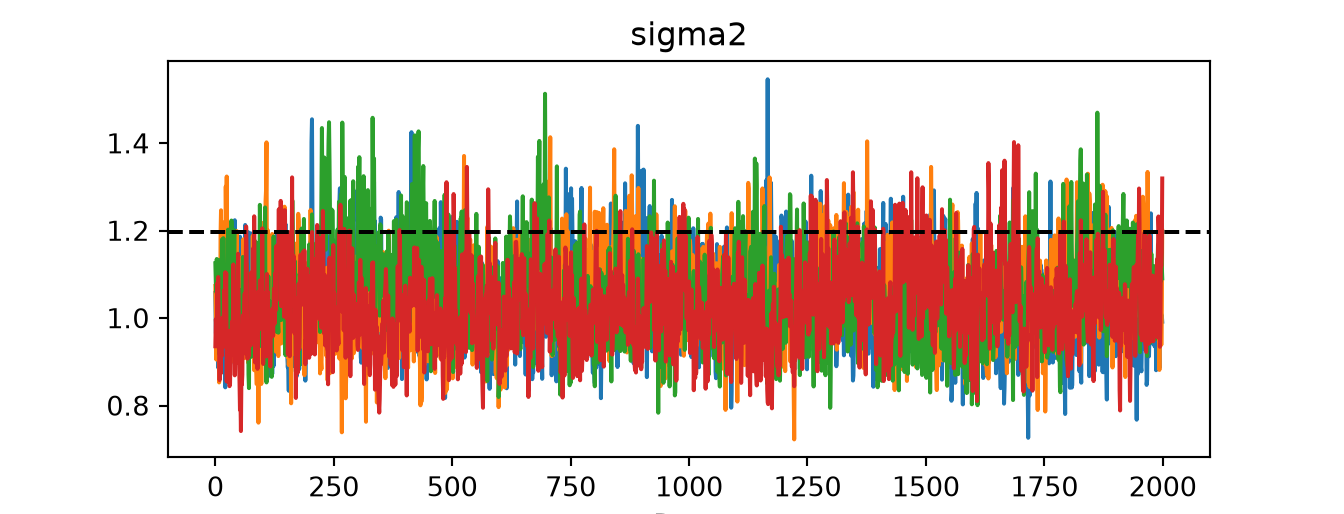

print("ESS:  ", az.ess(idata))

ESS:   <xarray.DataTree 'posterior'>
Group: /posterior
    Dimensions:  ()
    Data variables:
        sigma2   float64 8B 327.8

print("R-hat:", az.rhat(idata))

R-hat: <xarray.DataTree 'posterior'>
Group: /posterior
    Dimensions:  ()
    Data variables:
        sigma2   float64 8B 1.013

az.plot_autocorr(idata)

plt.show()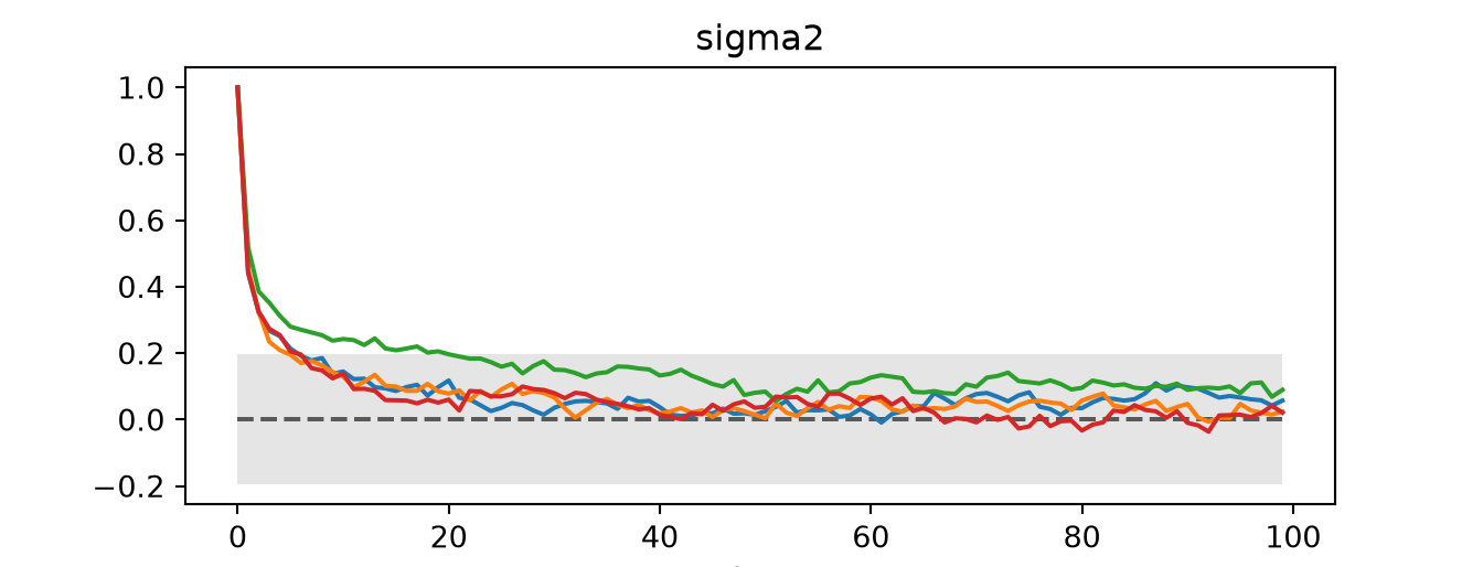

We can convert this to an array to be consumed by the bayesplot package.

R

coda_array <- as.array(sigma2_coda_list)
dim(coda_array) <- c(nrow(coda_array), ncol(coda_array), 1)
dimnames(coda_array) <- list(
  Iteration = paste0("iter", 1:num_mcmc),
  Chain = paste0("chain", 1:num_chains),
  Parameter = "sigma2_global"
)

Python

# sigma2_by_chain already has shape (num_chains, num_mcmc) — ready for per-chain plots
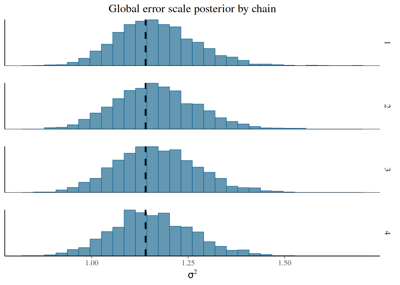
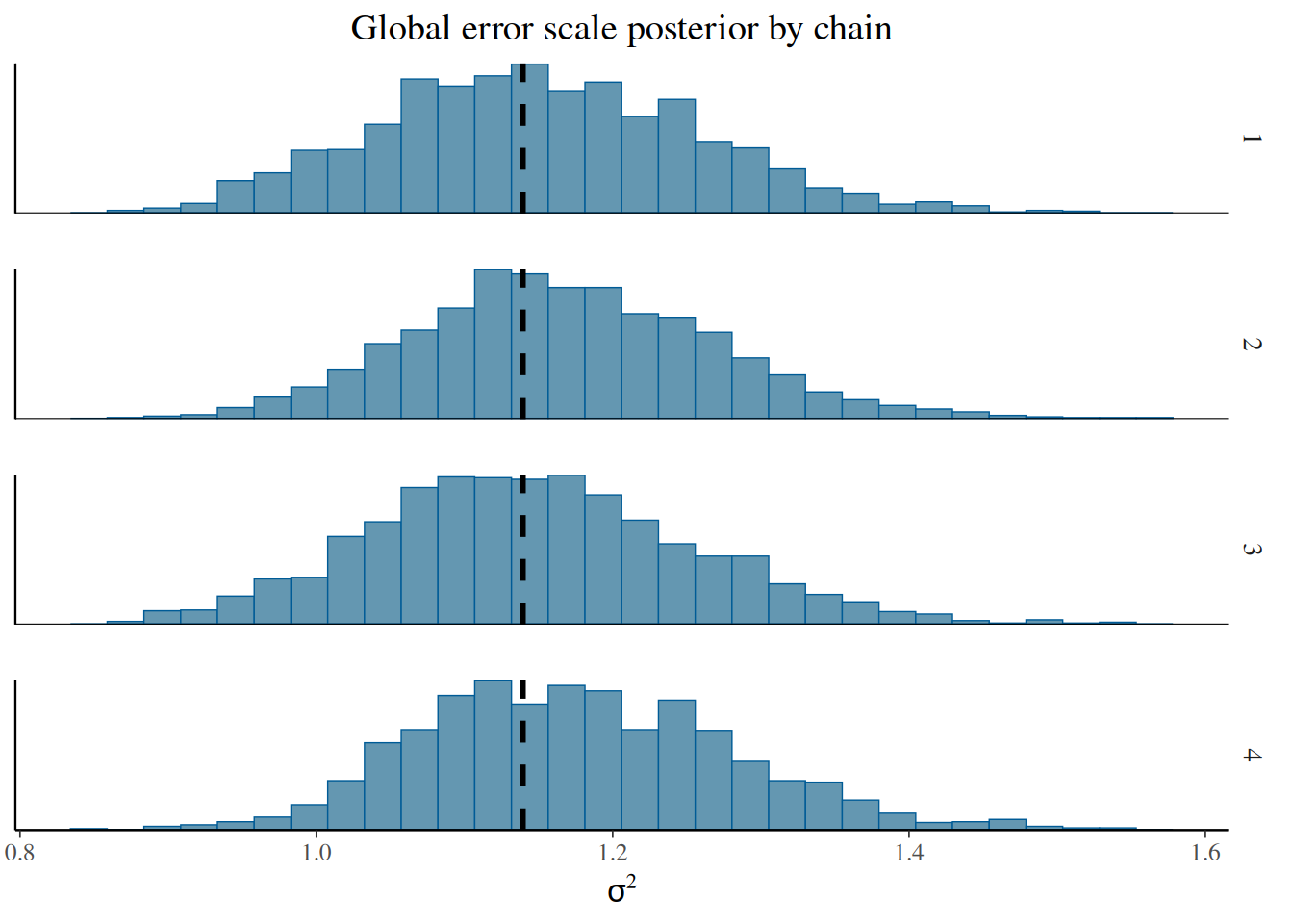
sigma2_chains = bart_model.global_var_samples.reshape(num_chains, num_mcmc)

<string>:2: DeprecationWarning: `BARTModel.global_var_samples` is deprecated and will be removed in a future release. The sampled values are owned by `model.samples`; use `model.extract_parameter("sigma2_global")` instead.

From here, we can visualize the posterior of \(\sigma^2\) for each chain, comparing to the true simulated value.

R

bayesplot::mcmc_hist_by_chain(
  coda_array,
  pars = "sigma2_global"
) +
  ggplot2::labs(
    title = "Global error scale posterior by chain",
    x = expression(sigma^2)
  ) +
  ggplot2::theme(
    plot.title = ggplot2::element_text(hjust = 0.5)
  ) +
  ggplot2::geom_vline(
    xintercept = noise_sd^2,
    color = "black",
    linetype = "dashed",
    size = 1
  )

Python

fig, axes = plt.subplots(1, num_chains, figsize=(12, 3), sharey=True)
for i, ax in enumerate(axes):
    ax.hist(sigma2_chains[i], bins=30)
    ax.axvline(noise_sd**2, color="black", linestyle="dashed", linewidth=1.5)
    ax.set_title(f"Chain {i+1}")
    ax.set_xlabel(r"$\sigma^2$")
fig.suptitle("Global error scale posterior by chain")
plt.tight_layout()
plt.show()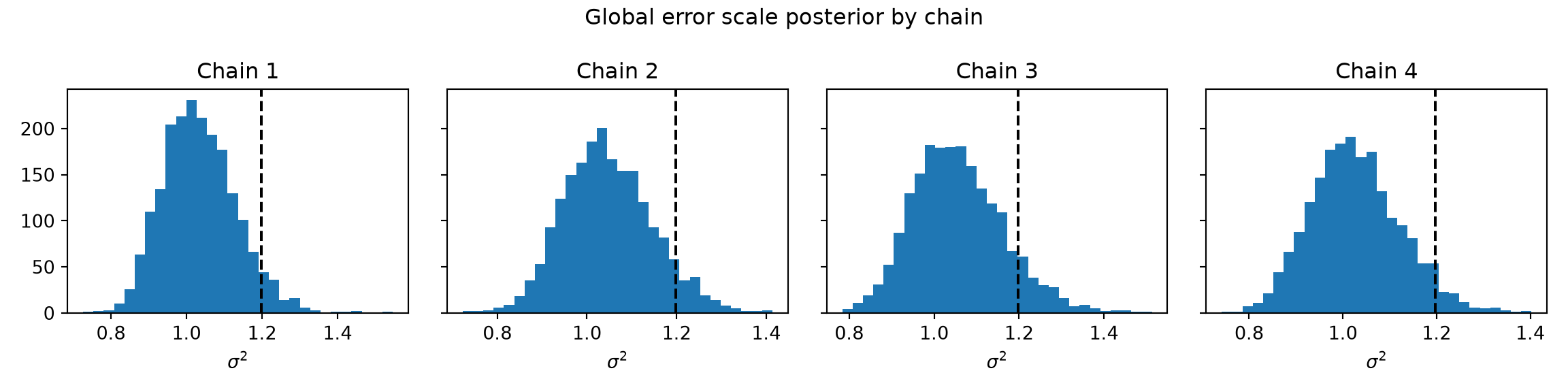

Sampling Multiple Chains Sequentially from XBART Forests

In the example above, each chain was initialized from “root”. If we sample a model using a small number of ‘grow-from-root’ iterations, we can use these forests to initialize MCMC chains.

R

num_chains <- 4
num_gfr <- 5
num_burnin <- 1000
num_mcmc <- 2000

Python

num_chains = 4
num_gfr    = 5
num_burnin = 1000
num_mcmc   = 2000

Run the initial GFR sampler.

R

xbart_model <- stochtree::bart(
  X_train = X_train,
  leaf_basis_train = leaf_basis_train,
  y_train = y_train,
  num_gfr = num_gfr,
  num_burnin = 0,
  num_mcmc = 0
)
xbart_model_string <- stochtree::saveBARTModelToJsonString(xbart_model)

Python

xbart_model = BARTModel()
xbart_model.sample(
    X_train=X_train, leaf_basis_train=leaf_basis_train, y_train=y_train,
    num_gfr=num_gfr, num_burnin=0, num_mcmc=0,
    general_params={"num_threads": 1},
)

BARTModel run with mean forest, global error variance model, and mean forest leaf scale model
Outcome was modeled as gaussian with a leaf regression prior with 1 bases for the mean forest
Outcome was standardized
The sampler was run for 5 GFR iterations, with 1 chain of 0 burn-in iterations and 0 MCMC iterations, retaining every iteration (i.e. no thinning)

xbart_model_json = xbart_model.to_json()

Run the multi-chain BART sampler, with each chain initialized from a different GFR forest.

R

bart_model <- stochtree::bart(
  X_train = X_train,
  leaf_basis_train = leaf_basis_train,
  y_train = y_train,
  num_gfr = num_gfr,
  num_burnin = num_burnin,
  num_mcmc = num_mcmc,
  general_params = list(num_chains = num_chains),
  previous_model_json = xbart_model_string,
  previous_model_warmstart_sample_num = num_gfr
)

Python

bart_model = BARTModel()
bart_model.sample(
    X_train=X_train, leaf_basis_train=leaf_basis_train, y_train=y_train,
    num_gfr=0, num_burnin=num_burnin, num_mcmc=num_mcmc,
    general_params={"num_threads": 1, "num_chains": num_chains},
    previous_model_json=xbart_model_json,
    previous_model_warmstart_sample_num=num_gfr - 1,  # 0-indexed
)

BARTModel run with mean forest, global error variance model, and mean forest leaf scale model
Outcome was modeled as gaussian with a leaf regression prior with 1 bases for the mean forest
Outcome was standardized
The sampler was run for 0 GFR iterations, with 4 chains of 1000 burn-in iterations and 2000 MCMC iterations, retaining every iteration (i.e. no thinning)

R

y_hat_test <- predict(
  bart_model,
  X = X_test,
  leaf_basis = leaf_basis_test,
  type = "mean",
  terms = "y_hat"
)
plot(y_hat_test, y_test, xlab = "Predicted", ylab = "Actual")
abline(0, 1, col = "red", lty = 3, lwd = 3)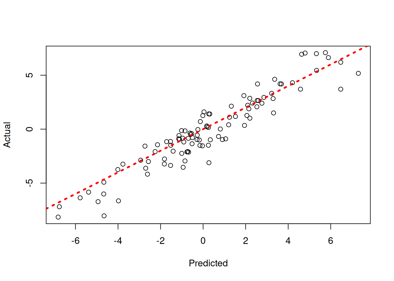

Python

y_hat_test = bart_model.predict(
    X=X_test, leaf_basis=leaf_basis_test, type="mean", terms="y_hat"
)
lo, hi = min(y_hat_test.min(), y_test.min()), max(y_hat_test.max(), y_test.max())
plt.scatter(y_hat_test, y_test, alpha=0.5)
plt.plot([lo, hi], [lo, hi], color="red", linestyle="dashed", linewidth=2)
plt.xlabel("Predicted"); plt.ylabel("Actual")
plt.show()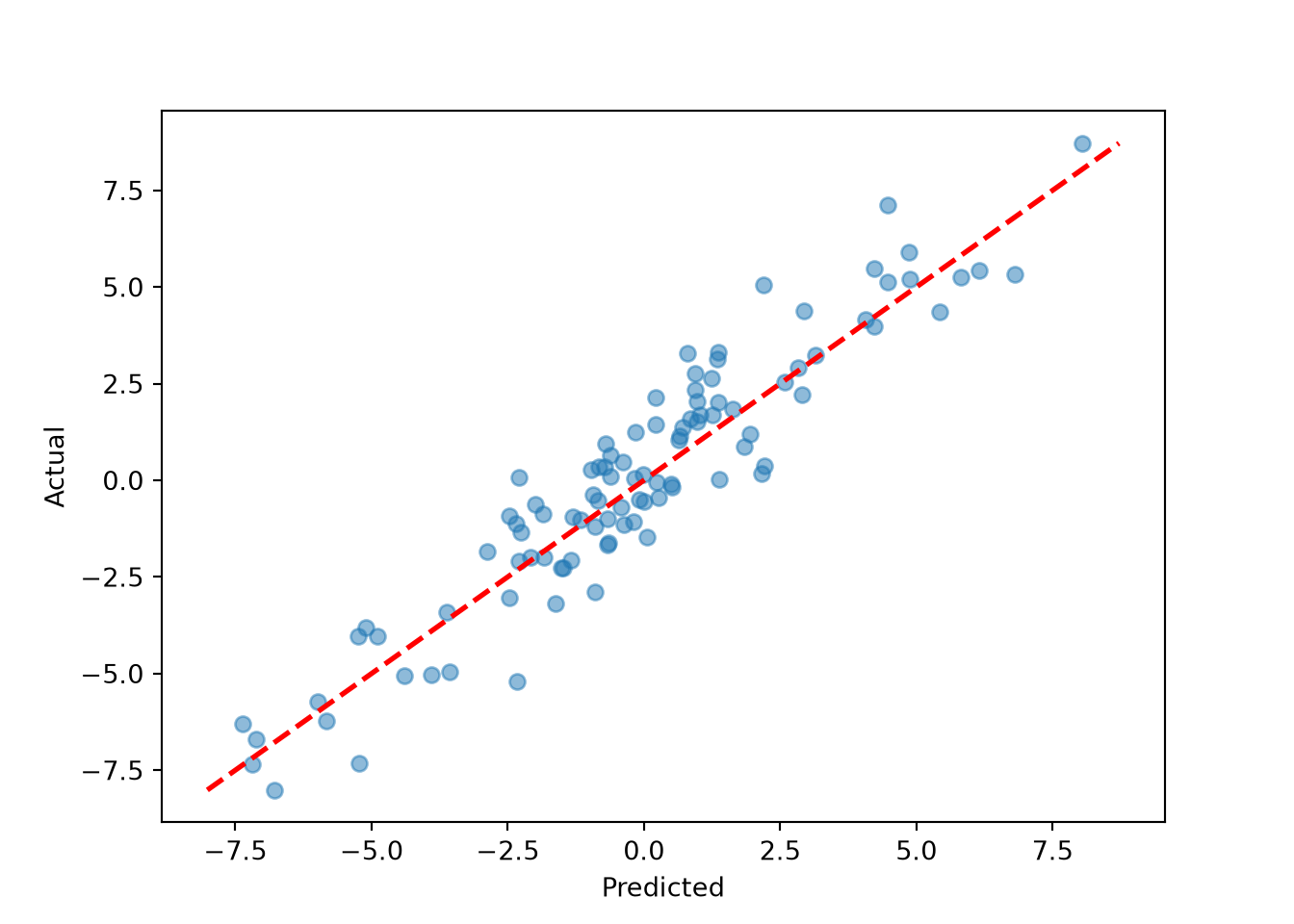

R

sigma2_coda_list <- coda::as.mcmc.list(lapply(
  1:num_chains,
  function(chain_idx) {
    offset <- (chain_idx - 1) * num_mcmc
    inds_start <- offset + 1
    inds_end <- offset + num_mcmc
    coda::mcmc(extractParameter(bart_model, "sigma2_global")[inds_start:inds_end])
  }
))
traceplot(sigma2_coda_list, ylab = expression(sigma^2))
abline(h = noise_sd^2, col = "black", lty = 3, lwd = 3)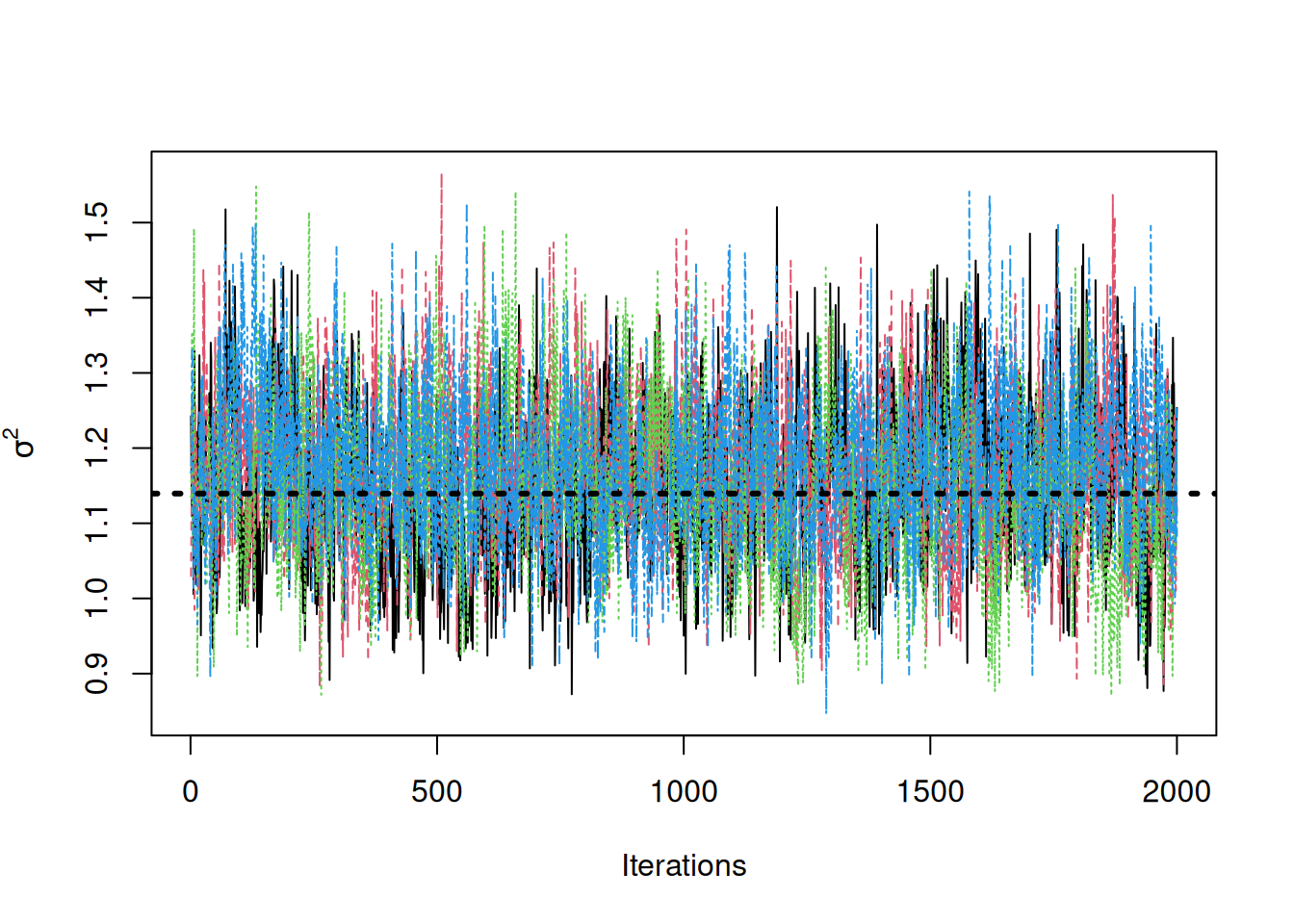

acf <- autocorr.diag(sigma2_coda_list)
ess <- effectiveSize(sigma2_coda_list)
rhat <- gelman.diag(sigma2_coda_list, autoburnin = F)
cat(paste0(
  "Average autocorrelation across chains:\n",
  paste0(paste0(rownames(acf), ": ", round(acf, 3)), collapse = ", "),
  "\nTotal effective sample size across chains: ",
  paste0(round(ess, 1), collapse = ", "),
  "\n'R-hat' potential scale reduction factor of Gelman and Rubin (1992)): ",
  paste0(round(rhat$psrf[, 1], 3), collapse = ", ")
))

Average autocorrelation across chains:
Lag 0: 1, Lag 1: 0.391, Lag 5: 0.166, Lag 10: 0.113, Lag 50: 0.022
Total effective sample size across chains: 1561
'R-hat' potential scale reduction factor of Gelman and Rubin (1992)): 1.012

Python

idata = az.from_dict({"posterior": {"sigma2": bart_model.global_var_samples.reshape(num_chains, num_mcmc)}})

<string>:1: DeprecationWarning: `BARTModel.global_var_samples` is deprecated and will be removed in a future release. The sampled values are owned by `model.samples`; use `model.extract_parameter("sigma2_global")` instead.

az.plot_trace(idata)

plt.axhline(noise_sd**2, color="black", linestyle="dashed", linewidth=1.5)
plt.show()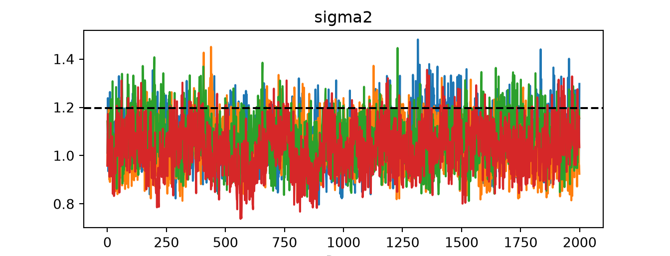

print("ESS:  ", az.ess(idata))

ESS:   <xarray.DataTree 'posterior'>
Group: /posterior
    Dimensions:  ()
    Data variables:
        sigma2   float64 8B 119.0

print("R-hat:", az.rhat(idata))

R-hat: <xarray.DataTree 'posterior'>
Group: /posterior
    Dimensions:  ()
    Data variables:
        sigma2   float64 8B 1.033

az.plot_autocorr(idata)

plt.show()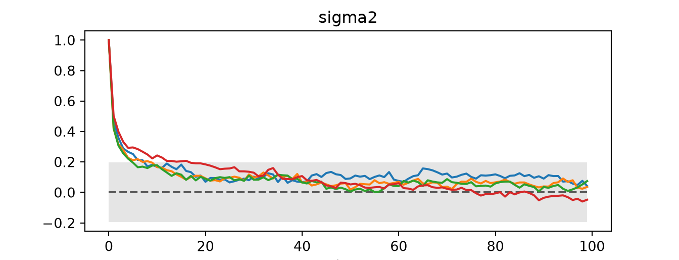

R

coda_array <- as.array(sigma2_coda_list)
dim(coda_array) <- c(nrow(coda_array), ncol(coda_array), 1)
dimnames(coda_array) <- list(
  Iteration = paste0("iter", 1:num_mcmc),
  Chain = paste0("chain", 1:num_chains),
  Parameter = "sigma2_global"
)

Python

sigma2_chains = bart_model.global_var_samples.reshape(num_chains, num_mcmc)

<string>:1: DeprecationWarning: `BARTModel.global_var_samples` is deprecated and will be removed in a future release. The sampled values are owned by `model.samples`; use `model.extract_parameter("sigma2_global")` instead.

R

bayesplot::mcmc_hist_by_chain(
  coda_array,
  pars = "sigma2_global"
) +
  ggplot2::labs(
    title = "Global error scale posterior by chain",
    x = expression(sigma^2)
  ) +
  ggplot2::theme(
    plot.title = ggplot2::element_text(hjust = 0.5)
  ) +
  ggplot2::geom_vline(
    xintercept = noise_sd^2,
    color = "black",
    linetype = "dashed",
    size = 1
  )

Python

fig, axes = plt.subplots(1, num_chains, figsize=(12, 3), sharey=True)
for i, ax in enumerate(axes):
    ax.hist(sigma2_chains[i], bins=30)
    ax.axvline(noise_sd**2, color="black", linestyle="dashed", linewidth=1.5)
    ax.set_title(f"Chain {i+1}")
    ax.set_xlabel(r"$\sigma^2$")
fig.suptitle("Global error scale posterior by chain")
plt.tight_layout()
plt.show()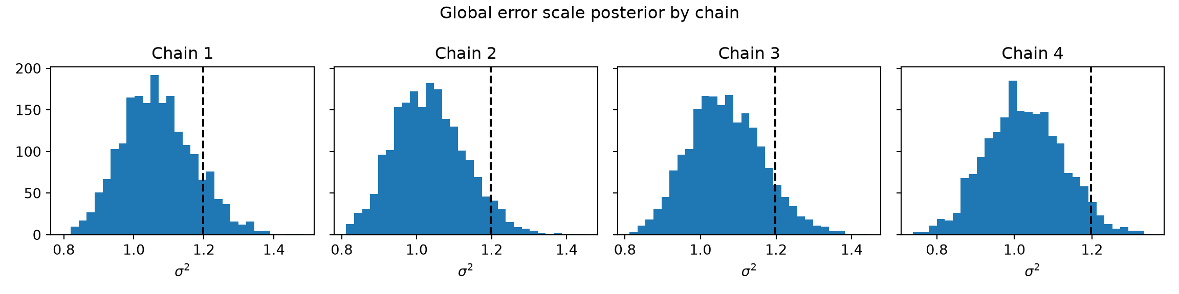

Sampling Multiple Chains in Parallel

While the above examples used sequential multi-chain sampling internally, it is also possible to run chains in parallel. In R, this is done via doParallel / foreach; in Python, via concurrent.futures.ProcessPoolExecutor. In both cases, each chain is serialized to JSON for cross-process communication, then combined into a single model via createBARTModelFromCombinedJsonString() (R) or BARTModel.from_json_string_list() (Python).

In order to run multiple parallel stochtree chains in R, a parallel backend must be registered. Note that we do not evaluate the cluster setup code below in order to interact nicely with GitHub Actions.

R

ncores <- parallel::detectCores()
cl <- makeCluster(ncores)
registerDoParallel(cl)

Python

# Worker function must be defined at module level for pickling
from concurrent.futures import ProcessPoolExecutor

def _run_bart_chain(args):
    X_tr, lb_tr, y_tr, X_te, lb_te, num_burnin, num_mcmc, seed = args
    from stochtree import BARTModel
    m = BARTModel()
    m.sample(
        X_train=X_tr, leaf_basis_train=lb_tr, y_train=y_tr,
        X_test=X_te, leaf_basis_test=lb_te,
        num_gfr=0, num_burnin=num_burnin, num_mcmc=num_mcmc,
        general_params={"num_threads": 1, "random_seed": seed},
        mean_forest_params={"sample_sigma2_leaf": False},
    )
    return m.to_json(), m.y_hat_test

R

num_chains <- 4
num_gfr <- 0
num_burnin <- 100
num_mcmc <- 100

Python

num_chains = 4
num_gfr    = 0
num_burnin = 100
num_mcmc   = 100

R

bart_model_outputs <- foreach(i = 1:num_chains) %dopar%
  {
    random_seed <- i
    general_params <- list(sample_sigma2_global = T, random_seed = random_seed)
    mean_forest_params <- list(sample_sigma2_leaf = F)
    bart_model <- stochtree::bart(
      X_train = X_train,
      leaf_basis_train = leaf_basis_train,
      y_train = y_train,
      X_test = X_test,
      leaf_basis_test = leaf_basis_test,
      num_gfr = num_gfr,
      num_burnin = num_burnin,
      num_mcmc = num_mcmc,
      general_params = general_params,
      mean_forest_params = mean_forest_params
    )
    bart_model_string <- stochtree::saveBARTModelToJsonString(bart_model)
    y_hat_test <- extractParameter(bart_model, "y_hat_test")
    list(model = bart_model_string, yhat = y_hat_test)
  }

Warning: executing %dopar% sequentially: no parallel backend registered

Python

# Sequential loop — replace the loop body with ProcessPoolExecutor for true parallelism
bart_model_outputs = []
for i in range(num_chains):
    m = BARTModel()
    m.sample(
        X_train=X_train, leaf_basis_train=leaf_basis_train, y_train=y_train,
        X_test=X_test, leaf_basis_test=leaf_basis_test,
        num_gfr=0, num_burnin=num_burnin, num_mcmc=num_mcmc,
        general_params={"num_threads": 1, "sample_sigma2_global": True, "random_seed": i + 1},
        mean_forest_params={"sample_sigma2_leaf": False},
    )
    bart_model_outputs.append({"model": m.to_json(), "yhat": m.y_hat_test})

BARTModel run with mean forest and global error variance model
Outcome was modeled as gaussian with a leaf regression prior with 1 bases for the mean forest
Outcome was standardized
The sampler was run for 0 GFR iterations, with 1 chain of 100 burn-in iterations and 100 MCMC iterations, retaining every iteration (i.e. no thinning)

<string>:10: DeprecationWarning: `BARTModel.y_hat_test` is deprecated and will be removed in a future release. The sampled values are owned by `model.samples`; use `model.extract_parameter("y_hat_test")` instead.
BARTModel run with mean forest and global error variance model
Outcome was modeled as gaussian with a leaf regression prior with 1 bases for the mean forest
Outcome was standardized
The sampler was run for 0 GFR iterations, with 1 chain of 100 burn-in iterations and 100 MCMC iterations, retaining every iteration (i.e. no thinning)

BARTModel run with mean forest and global error variance model
Outcome was modeled as gaussian with a leaf regression prior with 1 bases for the mean forest
Outcome was standardized
The sampler was run for 0 GFR iterations, with 1 chain of 100 burn-in iterations and 100 MCMC iterations, retaining every iteration (i.e. no thinning)

BARTModel run with mean forest and global error variance model
Outcome was modeled as gaussian with a leaf regression prior with 1 bases for the mean forest
Outcome was standardized
The sampler was run for 0 GFR iterations, with 1 chain of 100 burn-in iterations and 100 MCMC iterations, retaining every iteration (i.e. no thinning)

Close the parallel cluster (not evaluated here).

R

stopCluster(cl)

Python

# No explicit teardown required when using concurrent.futures context manager

Combine the forests from each BART model into a single forest.

R

bart_model_strings <- list()
bart_model_yhats <- matrix(NA, nrow = length(y_test), ncol = num_chains)
for (i in 1:length(bart_model_outputs)) {
  bart_model_strings[[i]] <- bart_model_outputs[[i]]$model
  bart_model_yhats[, i] <- rowMeans(bart_model_outputs[[i]]$yhat)
}
combined_bart <- createBARTModelFromCombinedJsonString(bart_model_strings)

Python

bart_model_strings = [out["model"] for out in bart_model_outputs]
bart_model_yhats = np.column_stack([
    out["yhat"].mean(axis=1) for out in bart_model_outputs
])  # shape: (n_test, num_chains)
combined_bart = BARTModel()
combined_bart.from_json_string_list(bart_model_strings)

R

yhat_combined <- predict(combined_bart, X_test, leaf_basis_test)$y_hat

Python

# type="posterior" (default) returns the full n_test × (num_chains * num_mcmc) matrix
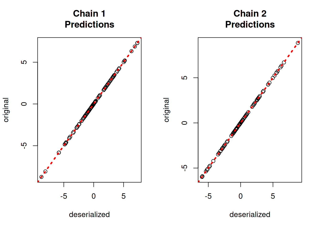
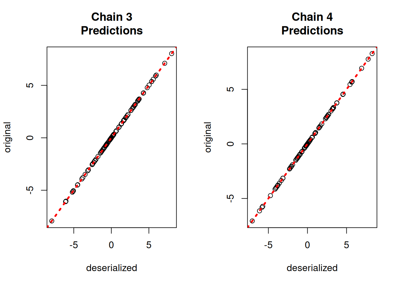
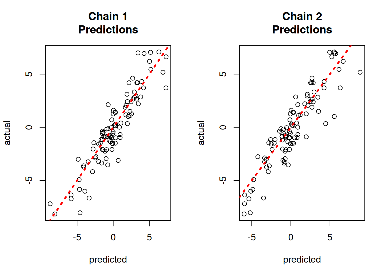
yhat_combined = combined_bart.predict(X=X_test, leaf_basis=leaf_basis_test, terms="y_hat")

Compare average predictions from each chain to the original predictions and to the true \(y\) values.

R

par(mfrow = c(1, 2))
for (i in 1:num_chains) {
  offset <- (i - 1) * num_mcmc
  inds_start <- offset + 1
  inds_end <- offset + num_mcmc
  plot(
    rowMeans(yhat_combined[, inds_start:inds_end]),
    bart_model_yhats[, i],
    xlab = "deserialized",
    ylab = "original",
    main = paste0("Chain ", i, "\nPredictions")
  )
  abline(0, 1, col = "red", lty = 3, lwd = 3)
}

par(mfrow = c(1, 1))

Python

fig, axes = plt.subplots(2, 2, figsize=(8, 8))
for i, ax in enumerate(axes.flat):
    chain_combined = yhat_combined[:, i * num_mcmc:(i + 1) * num_mcmc].mean(axis=1)
    chain_orig = bart_model_yhats[:, i]
    lo = min(chain_combined.min(), chain_orig.min())
    hi = max(chain_combined.max(), chain_orig.max())
    ax.scatter(chain_combined, chain_orig, alpha=0.4, s=10)
    ax.plot([lo, hi], [lo, hi], color="red", linestyle="dashed", linewidth=1.5)
    ax.set_xlabel("Deserialized"); ax.set_ylabel("Original")
    ax.set_title(f"Chain {i+1} Predictions")
plt.tight_layout()
plt.show()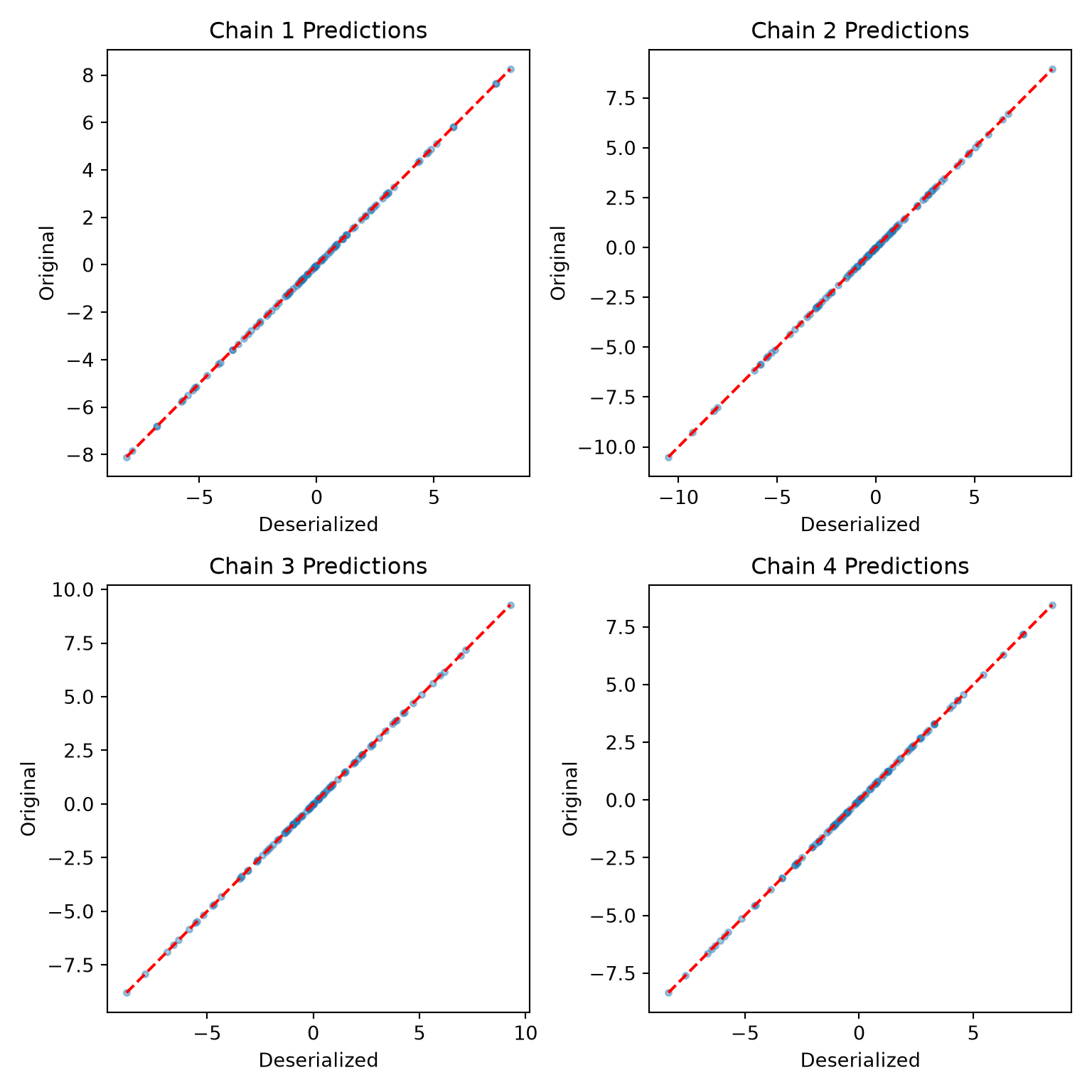

R

par(mfrow = c(1, 2))
for (i in 1:num_chains) {
  offset <- (i - 1) * num_mcmc
  inds_start <- offset + 1
  inds_end <- offset + num_mcmc
  plot(
    rowMeans(yhat_combined[, inds_start:inds_end]),
    y_test,
    xlab = "predicted",
    ylab = "actual",
    main = paste0("Chain ", i, "\nPredictions")
  )
  abline(0, 1, col = "red", lty = 3, lwd = 3)
}

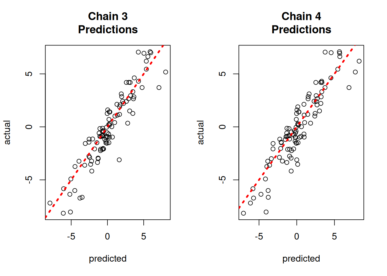
par(mfrow = c(1, 1))

Python

fig, axes = plt.subplots(2, 2, figsize=(8, 8))
for i, ax in enumerate(axes.flat):
    chain_pred = yhat_combined[:, i * num_mcmc:(i + 1) * num_mcmc].mean(axis=1)
    lo = min(chain_pred.min(), y_test.min())
    hi = max(chain_pred.max(), y_test.max())
    ax.scatter(chain_pred, y_test, alpha=0.4, s=10)
    ax.plot([lo, hi], [lo, hi], color="red", linestyle="dashed", linewidth=1.5)
    ax.set_xlabel("Predicted"); ax.set_ylabel("Actual")
    ax.set_title(f"Chain {i+1} Predictions")
plt.tight_layout()
plt.show()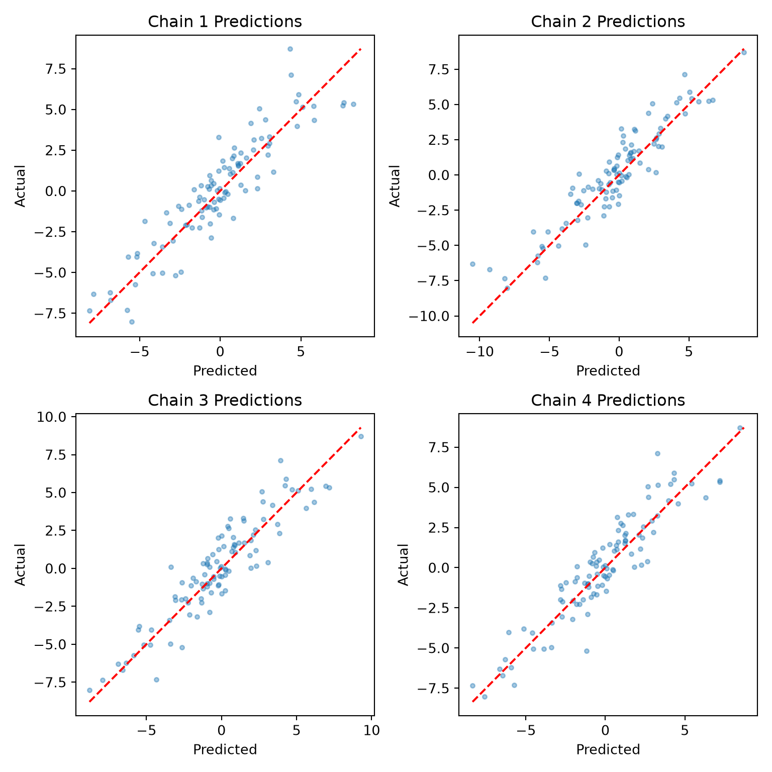

References

Chipman, Hugh A., Edward I. George, and Robert E. McCulloch. 2010. “BART: Bayesian additive regression trees.” The Annals of Applied Statistics 4 (1): 266–98. https://doi.org/10.1214/09-AOAS285.

He, Jingyu, and P Richard Hahn. 2023. “Stochastic Tree Ensembles for Regularized Nonlinear Regression.” Journal of the American Statistical Association 118 (541): 551–70.

Krantsevich, Nikolay, Jingyu He, and P Richard Hahn. 2023. “Stochastic Tree Ensembles for Estimating Heterogeneous Effects.” International Conference on Artificial Intelligence and Statistics, 6120–31.