Posterior Summary and Visualization Utilities

This vignette demonstrates the summary and plotting utilities available for stochtree models.

Setup

Load necessary packages

library(stochtree)

import numpy as np
import matplotlib.pyplot as plt
from stochtree import BARTModel, BCFModel, plot_parameter_trace

Set a seed for reproducibility

random_seed = 1234
set.seed(random_seed)

random_seed = 1234
rng = np.random.default_rng(random_seed)

Supervised Learning

We begin with the supervised learning use case served by the bart() function.

Below we simulate a simple regression dataset.

n <- 1000
p_x <- 10
p_w <- 1
X <- matrix(runif(n * p_x), ncol = p_x)
W <- matrix(runif(n * p_w), ncol = p_w)
f_XW <- (((0 <= X[, 10]) & (0.25 > X[, 10])) *
  (-7.5 * W[, 1]) +
  ((0.25 <= X[, 10]) & (0.5 > X[, 10])) * (-2.5 * W[, 1]) +
  ((0.5 <= X[, 10]) & (0.75 > X[, 10])) * (2.5 * W[, 1]) +
  ((0.75 <= X[, 10]) & (1 > X[, 10])) * (7.5 * W[, 1]))
noise_sd <- 1
y <- f_XW + rnorm(n, 0, 1) * noise_sd

n = 1000
p_x = 10
p_w = 1
X = rng.uniform(size=(n, p_x))
W = rng.uniform(size=(n, p_w))
# R uses X[,10] (1-indexed) = Python X[:,9]
f_XW = (
    ((X[:, 9] >= 0)    & (X[:, 9] < 0.25)) * (-7.5 * W[:, 0]) +
    ((X[:, 9] >= 0.25) & (X[:, 9] < 0.5))  * (-2.5 * W[:, 0]) +
    ((X[:, 9] >= 0.5)  & (X[:, 9] < 0.75)) * ( 2.5 * W[:, 0]) +
    ((X[:, 9] >= 0.75) & (X[:, 9] < 1.0))  * ( 7.5 * W[:, 0])
)
noise_sd = 1.0
y = f_XW + rng.standard_normal(n) * noise_sd

Now we fit a simple BART model to the data.

num_gfr <- 10
num_burnin <- 0
num_mcmc <- 1000
general_params <- list(
  num_threads = 1, 
  num_chains = 3
)
bart_model <- stochtree::bart(
  X_train = X,
  y_train = y,
  leaf_basis_train = W,
  num_gfr = num_gfr,
  num_burnin = num_burnin,
  num_mcmc = num_mcmc,
  general_params = general_params
)

bart_model = BARTModel()
bart_model.sample(
    X_train=X,
    y_train=y,
    leaf_basis_train=W,
    num_gfr=10,
    num_burnin=0,
    num_mcmc=1000,
    general_params={
      "num_threads": 1, 
      "num_chains": 3
    },
)

BARTModel run with mean forest, global error variance model, and mean forest leaf scale model
Outcome was modeled as gaussian with a leaf regression prior with 1 bases for the mean forest
Outcome was standardized
The sampler was run for 10 GFR iterations, with 3 chains of 0 burn-in iterations and 1000 MCMC iterations, retaining every iteration (i.e. no thinning)

We obtain a high level summary of the BART model by running print().

print(bart_model)

stochtree::bart() run with mean forest, global error variance model, and mean forest leaf scale model
Continuous outcome was modeled as Gaussian with a leaf regression prior with 1 bases for the mean forest
Outcome was standardized
The sampler was run for 10 GFR iterations, with 3 chains of 0 burn-in iterations and 1000 MCMC iterations, retaining every iteration (i.e. no thinning)

print(bart_model)

BARTModel run with mean forest, global error variance model, and mean forest leaf scale model
Outcome was modeled as gaussian with a leaf regression prior with 1 bases for the mean forest
Outcome was standardized
The sampler was run for 10 GFR iterations, with 3 chains of 0 burn-in iterations and 1000 MCMC iterations, retaining every iteration (i.e. no thinning)

For a more detailed summary (including the information above), we use the summary() function.

summary(bart_model)

stochtree::bart() run with mean forest, global error variance model, and mean forest leaf scale model
Continuous outcome was modeled as Gaussian with a leaf regression prior with 1 bases for the mean forest
Outcome was standardized
The sampler was run for 10 GFR iterations, with 3 chains of 0 burn-in iterations and 1000 MCMC iterations, retaining every iteration (i.e. no thinning) 
Summary of sigma^2 posterior: 
3000 samples, mean = 0.883, standard deviation = 0.048, quantiles:
     2.5%       10%       25%       50%       75%       90%     97.5% 
0.7931489 0.8220718 0.8505011 0.8803660 0.9142145 0.9449494 0.9805524 
Summary of leaf scale posterior: 
3000 samples, mean = 0.008, standard deviation = 0.003, quantiles:
       2.5%         10%         25%         50%         75%         90% 
0.005098496 0.005839803 0.006598690 0.007495546 0.008618220 0.010803190 
      97.5% 
0.016509682 
Summary of in-sample posterior mean predictions: 
1000 observations, mean = -0.064, standard deviation = 3.287, quantiles:
      2.5%        10%        25%        50%        75%        90%      97.5% 
-6.8629988 -4.9589880 -1.8446658 -0.1196631  2.0197249  4.2943567  6.5781901

print(bart_model.summary())

BART Model Summary:
-------------------
BARTModel run with mean forest, global error variance model, and mean forest leaf scale model
Outcome was modeled as gaussian with a leaf regression prior with 1 bases for the mean forest
Outcome was standardized
The sampler was run for 10 GFR iterations, with 3 chains of 0 burn-in iterations and 1000 MCMC iterations, retaining every iteration (i.e. no thinning)

Summary of sigma^2 posterior: 3000 samples, mean = 0.929, standard deviation = 0.050, quantiles:
    2.5%: 0.836
   10.0%: 0.867
   25.0%: 0.895
   50.0%: 0.927
   75.0%: 0.961
   90.0%: 0.994
   97.5%: 1.031
Summary of leaf scale posterior: 3000 samples, mean = 0.008, standard deviation = 0.002, quantiles:
    2.5%: 0.006
   10.0%: 0.007
   25.0%: 0.007
   50.0%: 0.008
   75.0%: 0.009
   90.0%: 0.010
   97.5%: 0.015
Summary of in-sample posterior mean predictions: 
1000 observations, mean = 0.106, standard deviation = 3.290, quantiles:
    2.5%: -6.767
   10.0%: -4.323
   25.0%: -1.939
   50.0%: 0.170
   75.0%: 2.093
   90.0%: 4.406
   97.5%: 6.588

None

We can use the plot() function to produce a traceplot of model terms like the global error scale \(\sigma^2\) or (if \(\sigma^2\) is not sampled) the first observation of cached train set predictions.

plot(bart_model)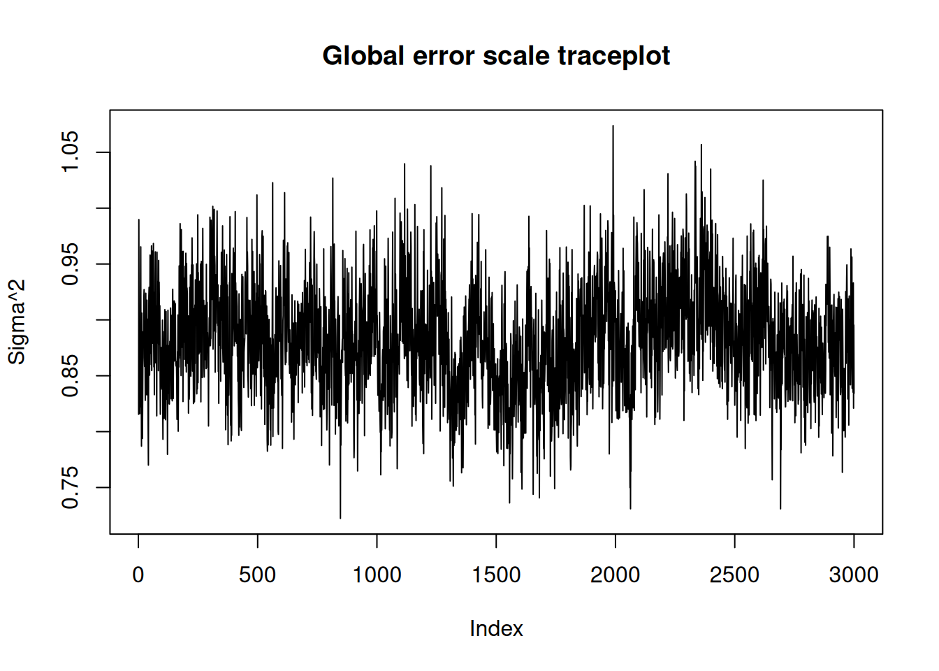

ax = plot_parameter_trace(bart_model, term="global_error_scale")
plt.show()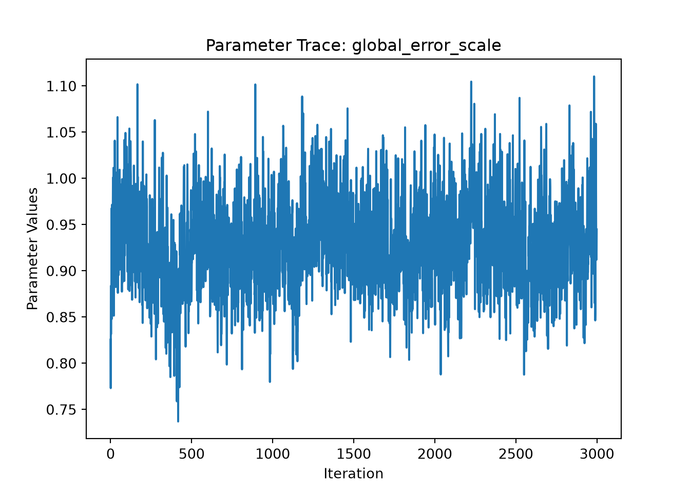

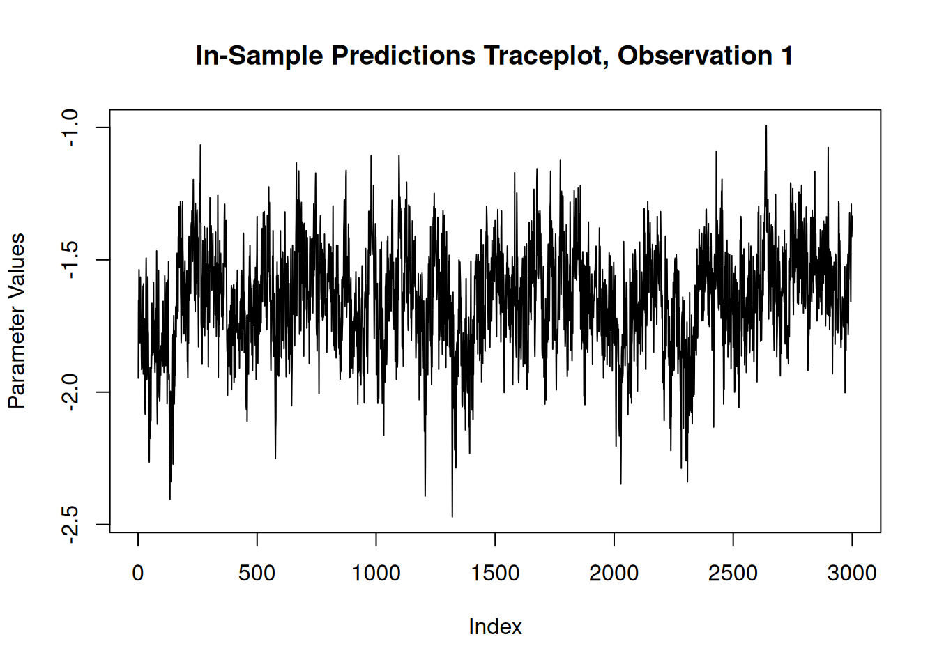
For finer-grained control over which parameters to plot, we can also use the extractParameter() function to pull the posterior distribution of any valid model term (e.g., global error scale \(\sigma^2\), leaf scale \(\sigma^2_{\ell}\), in-sample mean function predictions y_hat_train) and then plot any subset or transformation of these values.

y_hat_train_samples <- extractParameter(bart_model, "y_hat_train")
obs_index <- 1
plot(
  y_hat_train_samples[obs_index, ],
  type = "l",
  main = paste0("In-Sample Predictions Traceplot, Observation ", obs_index),
  xlab = "Index",
  ylab = "Parameter Values"
)

y_hat_train_samples = bart_model.extract_parameter("y_hat_train")
obs_index = 0
fig, ax = plt.subplots()
ax.plot(y_hat_train_samples[obs_index, :])
ax.set_title(f"In-Sample Predictions Traceplot, Observation {obs_index}")
ax.set_xlabel("Index")
ax.set_ylabel("Parameter Values")
plt.show()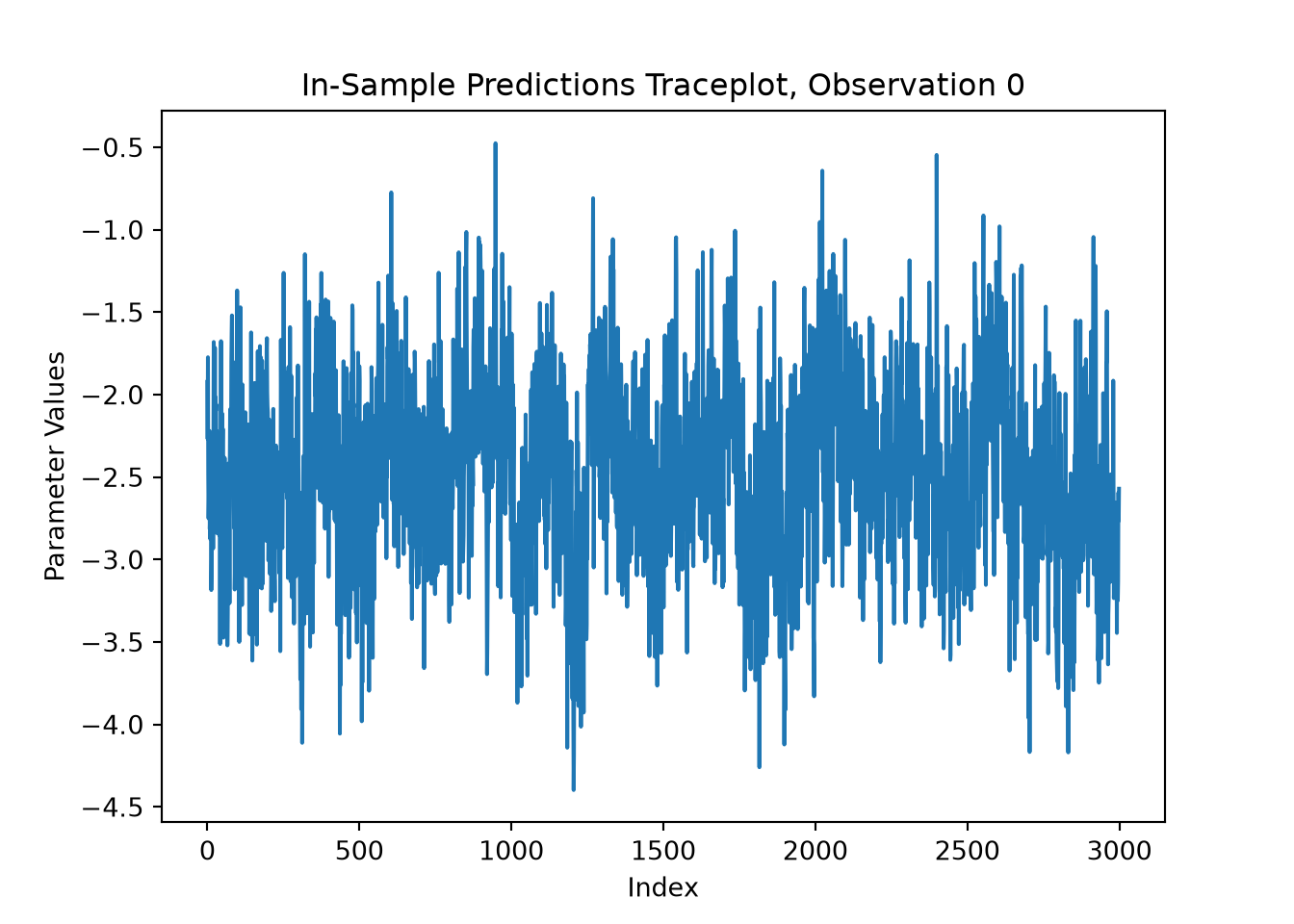

Causal Inference

We now run the same demo for the causal inference use case served by the bcf() function in R and the BCFModel Python class.

Below we simulate a simple dataset for a causal inference problem with binary treatment and continuous outcome.

# Generate covariates and treatment
n <- 1000
p_X = 5
X = matrix(runif(n * p_X), ncol = p_X)
pi_X = 0.25 + 0.5 * X[, 1]
Z = rbinom(n, 1, pi_X)

# Define the outcome mean functions (prognostic and treatment effects)
mu_X = pi_X * 5 + 2 * X[, 3]
tau_X = X[, 2] * 2 - 1

# Generate outcome
epsilon = rnorm(n, 0, 1)
y = mu_X + tau_X * Z + epsilon

# Generate covariates and treatment
n = 1000
p_X = 5
X = rng.uniform(size=(n, p_X))
pi_X = 0.25 + 0.5 * X[:, 0]
Z = rng.binomial(1, pi_X, n).astype(float)

# Define the outcome mean functions (prognostic and treatment effects)
mu_X = pi_X * 5 + 2 * X[:, 2]
tau_X = X[:, 1] * 2 - 1

# Generate outcome
epsilon = rng.standard_normal(n)
y = mu_X + tau_X * Z + epsilon

Now we fit a simple BCF model to the data

num_gfr <- 10
num_burnin <- 0
num_mcmc <- 1000
general_params <- list(
  num_threads = 1, 
  num_chains = 3, 
  adaptive_coding = TRUE
)
bcf_model <- stochtree::bcf(
  X_train = X,
  y_train = y,
  Z_train = Z,
  num_gfr = num_gfr,
  num_burnin = num_burnin,
  num_mcmc = num_mcmc,
  general_params = general_params
)

bcf_model = BCFModel()
bcf_model.sample(
    X_train=X,
    Z_train=Z,
    y_train=y,
    propensity_train=pi_X,
    num_gfr=10,
    num_burnin=0,
    num_mcmc=1000,
    general_params={
      "num_threads": 1, 
      "num_chains": 3, 
      "adaptive_coding": True
    },
)

BCFModel run with prognostic forest, treatment effect forest, global error variance model, prognostic forest leaf scale model, and treatment effect intercept model
Outcome was modeled as gaussian
Treatment was binary and its effect was estimated with adaptive coding
Outcome was standardized
User-provided propensity scores were included in the model
The sampler was run for 10 GFR iterations, with 3 chains of 0 burn-in iterations and 1000 MCMC iterations, retaining every iteration (i.e. no thinning)

We obtain a high level summary of the BCF model by running print().

print(bcf_model)

stochtree::bcf() run with prognostic forest, treatment effect forest, global error variance model, prognostic forest leaf scale model, and treatment effect intercept model
Outcome was modeled as gaussian
Treatment was binary and its effect was estimated with adaptive coding
outcome was standardized
An internal propensity model was fit using stochtree::bart() in lieu of user-provided propensity scores
The sampler was run for 10 GFR iterations, with 3 chains of 0 burn-in iterations and 1000 MCMC iterations, retaining every iteration (i.e. no thinning)

print(bcf_model)

BCFModel run with prognostic forest, treatment effect forest, global error variance model, prognostic forest leaf scale model, and treatment effect intercept model
Outcome was modeled as gaussian
Treatment was binary and its effect was estimated with adaptive coding
Outcome was standardized
User-provided propensity scores were included in the model
The sampler was run for 10 GFR iterations, with 3 chains of 0 burn-in iterations and 1000 MCMC iterations, retaining every iteration (i.e. no thinning)

For a more detailed summary (including the information above), we use the summary() function / method.

summary(bcf_model)

stochtree::bcf() run with prognostic forest, treatment effect forest, global error variance model, prognostic forest leaf scale model, and treatment effect intercept model
Outcome was modeled as gaussian
Treatment was binary and its effect was estimated with adaptive coding
outcome was standardized
An internal propensity model was fit using stochtree::bart() in lieu of user-provided propensity scores
The sampler was run for 10 GFR iterations, with 3 chains of 0 burn-in iterations and 1000 MCMC iterations, retaining every iteration (i.e. no thinning) 
Summary of sigma^2 posterior: 
3000 samples, mean = 0.952, standard deviation = 0.045, quantiles:
     2.5%       10%       25%       50%       75%       90%     97.5% 
0.8684495 0.8945314 0.9211950 0.9516468 0.9811881 1.0096271 1.0420225 
Summary of prognostic forest leaf scale posterior: 
3000 samples, mean = 0.001, standard deviation = 0.000, quantiles:
        2.5%          10%          25%          50%          75%          90% 
0.0009254776 0.0010823268 0.0012293533 0.0014456313 0.0016757870 0.0019007878 
       97.5% 
0.0021630332 
Summary of adaptive coding parameters: 
3000 samples, mean (control) = -0.288, mean (treated) = 0.838, standard deviation (control) = 0.285, standard deviation (treated) = 0.255
quantiles (control):
       2.5%         10%         25%         50%         75%         90% 
-0.92315576 -0.65333296 -0.44728393 -0.27083095 -0.10015099  0.04447522 
      97.5% 
 0.21149015 
quantiles (treated):
     2.5%       10%       25%       50%       75%       90%     97.5% 
0.3737871 0.5121534 0.6537976 0.8339336 1.0078002 1.1706313 1.3623031 
Summary of treatment effect intercept (tau_0) posterior: 
3000 samples, mean = -0.298, standard deviation = 0.584, quantiles:
      2.5%        10%        25%        50%        75%        90%      97.5% 
-1.3862066 -1.1283068 -0.7625600 -0.2613363  0.1786662  0.4629315  0.6312075 
Summary of in-sample posterior mean predictions: 
1000 observations, mean = 3.488, standard deviation = 0.944, quantiles:
    2.5%      10%      25%      50%      75%      90%    97.5% 
1.677978 2.290777 2.821136 3.478399 4.129673 4.729020 5.409691 
Summary of in-sample posterior mean CATEs: 
1000 observations, mean = 0.074, standard deviation = 0.521, quantiles:
        2.5%          10%          25%          50%          75%          90% 
-0.746811465 -0.563293994 -0.387421722  0.002999033  0.576887755  0.779291612 
       97.5% 
 0.903682476

print(bcf_model.summary())

BCF Model Summary:
------------------
BCFModel run with prognostic forest, treatment effect forest, global error variance model, prognostic forest leaf scale model, and treatment effect intercept model
Outcome was modeled as gaussian
Treatment was binary and its effect was estimated with adaptive coding
Outcome was standardized
User-provided propensity scores were included in the model
The sampler was run for 10 GFR iterations, with 3 chains of 0 burn-in iterations and 1000 MCMC iterations, retaining every iteration (i.e. no thinning)

Summary of sigma^2 posterior: 3000 samples, mean = 0.873, standard deviation = 0.043, quantiles:
    2.5%: 0.790
   10.0%: 0.820
   25.0%: 0.844
   50.0%: 0.872
   75.0%: 0.900
   90.0%: 0.929
   97.5%: 0.963
Summary of prognostic forest leaf scale posterior: 3000 samples, mean = 0.002, standard deviation = 0.000, quantiles:
    2.5%: 0.001
   10.0%: 0.001
   25.0%: 0.001
   50.0%: 0.002
   75.0%: 0.002
   90.0%: 0.002
   97.5%: 0.002
Summary of adaptive coding parameters: 
3000 samples, mean (control) = -0.367, mean (treated) = 0.946, standard deviation (control) = 0.281, standard deviation (treated) = 0.291
quantiles (control):
    2.5%: -0.945
   10.0%: -0.746
   25.0%: -0.544
   50.0%: -0.345
   75.0%: -0.172
   90.0%: -0.032
   97.5%: 0.137

quantiles (treated):
    2.5%: 0.427
   10.0%: 0.573
   25.0%: 0.732
   50.0%: 0.938
   75.0%: 1.142
   90.0%: 1.328
   97.5%: 1.536
Summary of treatment effect intercept (tau_0) posterior: 3000 samples, mean = -0.078, standard deviation = 0.410, quantiles:
    2.5%: -0.852
   10.0%: -0.600
   25.0%: -0.369
   50.0%: -0.080
   75.0%: 0.213
   90.0%: 0.475
   97.5%: 0.701
Summary of in-sample posterior mean predictions: 
1000 observations, mean = 3.482, standard deviation = 0.960, quantiles:
    2.5%: 1.850
   10.0%: 2.215
   25.0%: 2.769
   50.0%: 3.465
   75.0%: 4.161
   90.0%: 4.770
   97.5%: 5.321
Summary of in-sample posterior mean CATEs: 
1000 observations, mean = -0.027, standard deviation = 0.632, quantiles:
    2.5%: -1.108
   10.0%: -0.941
   25.0%: -0.568
   50.0%: 0.061
   75.0%: 0.537
   90.0%: 0.752
   97.5%: 0.935

None

In R, we have a plot() that produces a traceplot of model terms like the global error scale \(\sigma^2\) or (if \(\sigma^2\) is not sampled) the first observation of cached train set predictions.

In Python, we provide a plot_parameter_trace() function for requesting a traceplot of a specific model parameter.

plot(bcf_model)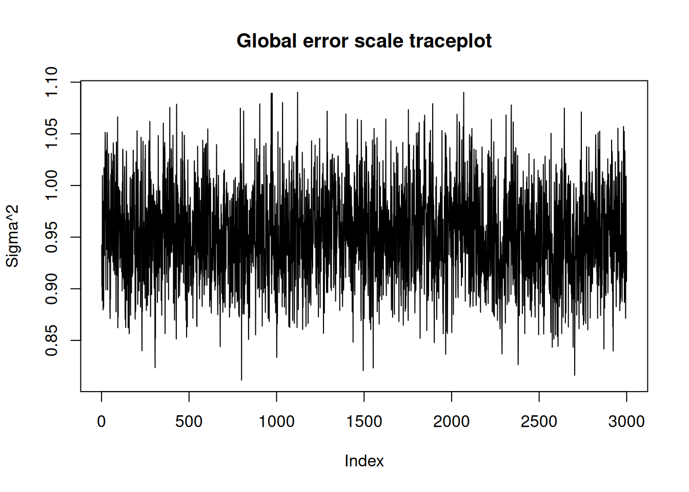

ax = plot_parameter_trace(bcf_model, term="global_error_scale")
plt.show()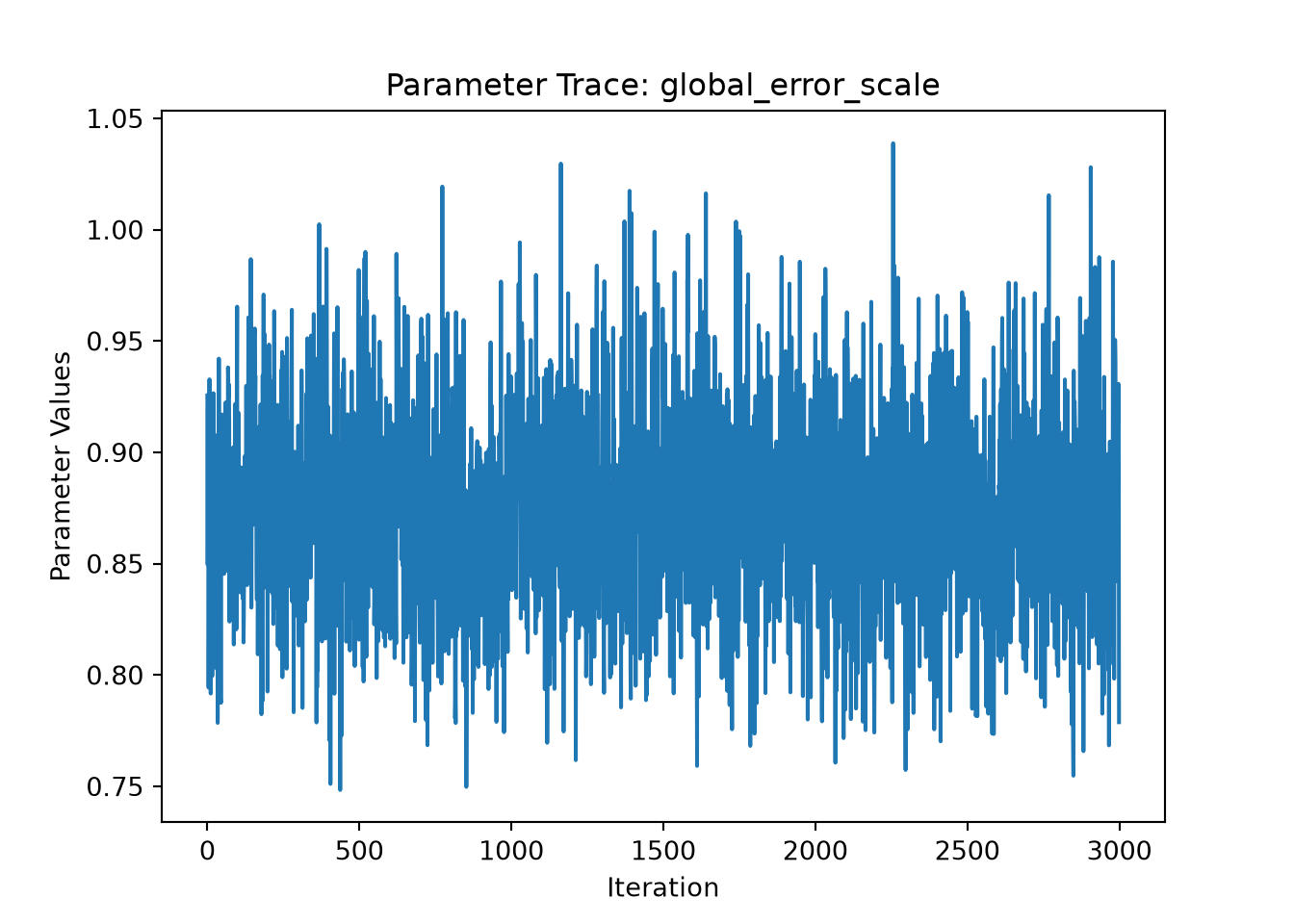

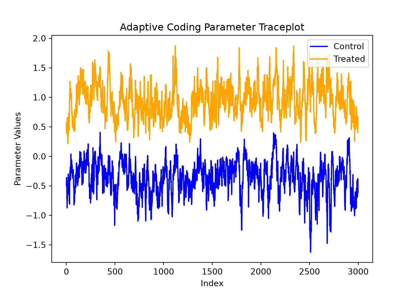
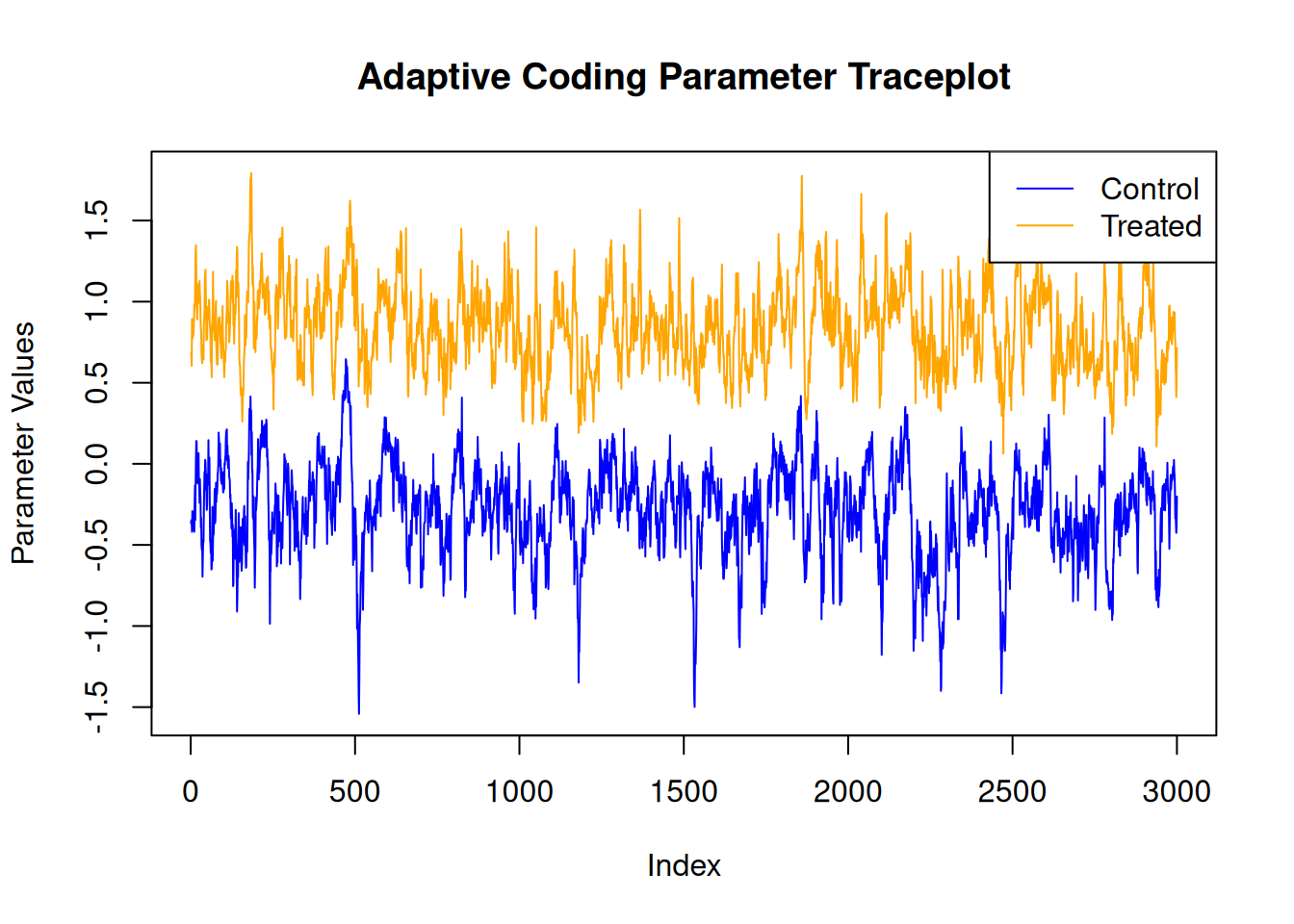
For finer-grained control over which parameters to plot, we can also use the extractParameter() function in R or the extract_parameter() method in Python to query the posterior distribution of any valid model term (e.g., global error scale \(\sigma^2\), prognostic forest leaf scale \(\sigma^2_{\mu}\), CATE forest leaf scale \(\sigma^2_{\tau}\), adaptive coding parameters \(b_0\) and \(b_1\) for binary treatment, in-sample mean function predictions y_hat_train, in-sample CATE function predictions tau_hat_train) and then plot any subset or transformation of these values.

adaptive_coding_samples <- extractParameter(bcf_model, "adaptive_coding")
plot(
  adaptive_coding_samples[1, ],
  type = "l",
  main = "Adaptive Coding Parameter Traceplot",
  xlab = "Index",
  ylab = "Parameter Values",
  ylim = range(adaptive_coding_samples),
  col = "blue"
)
lines(adaptive_coding_samples[2, ], col = "orange")
legend(
  "topright",
  legend = c("Control", "Treated"),
  lty = 1,
  col = c("blue", "orange")
)

adaptive_coding_samples = bcf_model.extract_parameter("adaptive_coding")
fig, ax = plt.subplots()
ax.plot(adaptive_coding_samples[0, :], color="blue", label="Control")
ax.plot(adaptive_coding_samples[1, :], color="orange", label="Treated")
ax.set_title("Adaptive Coding Parameter Traceplot")
ax.set_xlabel("Index")
ax.set_ylabel("Parameter Values")
ax.legend(loc="upper right")
plt.show()