BCF with Vector-valued Treatments

BCF extended to vector-valued (multivariate) treatments, estimating heterogeneous effects for multiple treatment arms simultaneously.

Background

When treatments are multivariate — such as continuous dose vectors or multiple binary arms — the standard BCF model extends to

\[ Y_i = \mu(X_i) + \tau(X_i)^\top Z_i + \epsilon_i \]

where \(Z_i \in \mathbb{R}^p\) and \(\tau(X_i) \in \mathbb{R}^p\) is a vector of covariate-dependent treatment effects.

Setup

Load necessary packages

R

library(stochtree)

Python

import matplotlib.pyplot as plt
import numpy as np
from sklearn.model_selection import train_test_split
from stochtree import BCFModel

Set a seed for reproducibility

R

random_seed <- 4321
set.seed(random_seed)

Python

random_seed = 4321
rng = np.random.default_rng(random_seed)

Data Simulation

R

# Generate covariates, propensities, and treatments
n <- 1000
p_X <- 5
X <- matrix(runif(n * p_X), nrow = n, ncol = p_X)
pi_X <- cbind(0.25 + 0.5 * X[, 1], 0.75 - 0.5 * X[, 2])
Z <- cbind(
  as.numeric(rbinom(n, 1, pi_X[, 1])),
  as.numeric(rbinom(n, 1, pi_X[, 2]))
)

# Define outcome mean functions (prognostic and treatment effects)
mu_X <- pi_X[, 1] * 5 + pi_X[, 2] * 2 + 2 * X[, 3]
tau_X <- cbind(X[, 2], X[, 3])

# Generate outcome
treatment_term <- rowSums(tau_X * Z)
y <- mu_X + treatment_term + rnorm(n)

Python

# Generate covariates, propensities, and treatments
n = 1000
p_X = 5
X = rng.uniform(0, 1, (n, p_X))
pi_X = np.c_[0.25 + 0.5 * X[:, 0], 0.75 - 0.5 * X[:, 1]]
Z = rng.binomial(1, pi_X, (n, 2)).astype(float)

# Define the outcome mean functions (prognostic and treatment effects)
mu_X = pi_X[:, 0] * 5 + pi_X[:, 1] * 2 + 2 * X[:, 2]
tau_X = np.stack((X[:, 1], X[:, 2]), axis=-1)

# Generate outcome
epsilon = rng.normal(0, 1, n)
treatment_term = np.multiply(tau_X, Z).sum(axis=1)
y = mu_X + treatment_term + epsilon

Split the data into train and test sets

R

n_test <- round(n * 0.2)
test_inds <- sort(sample(seq_len(n), n_test, replace = FALSE))
train_inds <- setdiff(seq_len(n), test_inds)
X_train <- X[train_inds, ]
X_test <- X[test_inds, ]
Z_train <- Z[train_inds, ]
Z_test <- Z[test_inds, ]
y_train <- y[train_inds]
y_test <- y[test_inds]
pi_train <- pi_X[train_inds, ]
pi_test <- pi_X[test_inds, ]
mu_train <- mu_X[train_inds]
mu_test <- mu_X[test_inds]
tau_train <- tau_X[train_inds, ]
tau_test <- tau_X[test_inds, ]

Python

sample_inds = np.arange(n)
train_inds, test_inds = train_test_split(sample_inds, test_size=0.2)
X_train = X[train_inds, :]
X_test = X[test_inds, :]
Z_train = Z[train_inds, :]
Z_test = Z[test_inds, :]
y_train = y[train_inds]
y_test = y[test_inds]
pi_train = pi_X[train_inds]
pi_test = pi_X[test_inds]
mu_train = mu_X[train_inds]
mu_test = mu_X[test_inds]
tau_train = tau_X[train_inds, :]
tau_test = tau_X[test_inds, :]

Model Fitting

Fit a multivariate BCF model

R

general_params <- list(
  num_threads = 1, 
  num_chains = 4,
  random_seed = random_seed, 
  adaptive_coding = FALSE
)
bcf_model <- bcf(
  X_train = X_train,
  Z_train = Z_train,
  y_train = y_train,
  propensity_train = pi_train,
  num_gfr = 10,
  num_burnin = 500,
  num_mcmc = 100, 
  general_params = general_params
)

Python

general_params = {
  "num_threads": 1,
  "num_chains": 4,
  "random_seed": random_seed, 
  "adaptive_coding": False
}
bcf_model = BCFModel()
bcf_model.sample(
    X_train=X_train,
    Z_train=Z_train,
    y_train=y_train,
    propensity_train=pi_train,
    num_gfr=10,
    num_burnin=500,
    num_mcmc=100,
    general_params=general_params,
)

BCFModel run with prognostic forest, treatment effect forest, global error variance model, prognostic forest leaf scale model, and treatment effect intercept model
Outcome was modeled as gaussian
Treatment was multivariate with 2 dimensions
Outcome was standardized
User-provided propensity scores were included in the model
The sampler was run for 10 GFR iterations, with 4 chains of 500 burn-in iterations and 100 MCMC iterations, retaining every iteration (i.e. no thinning)

Posterior Summaries

Compare true outcomes to predicted conditional means

R

y_hat_test <- predict(
  bcf_model,
  X = X_test,
  Z = Z_test,
  propensity = pi_test,
  terms = "y_hat",
  type = "mean"
)
plot(
  y_hat_test,
  y_test,
  xlab = "Average estimated outcome",
  ylab = "True outcome"
)
abline(0, 1, col = "black", lty = 3)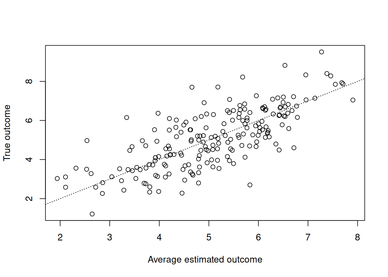

rmse <- sqrt(mean((y_hat_test - y_test)^2))
cat("Test-set RMSE: ", rmse, "\n")

Test-set RMSE:  1.030903 

Python

y_hat_test = bcf_model.predict(
    X=X_test, Z=Z_test, propensity=pi_test, terms="y_hat", type="mean"
)
lo, hi = min(y_hat_test.min(), y_test.min()), max(y_hat_test.max(), y_test.max())
plt.scatter(y_hat_test, y_test, alpha=0.5)
plt.plot([lo, hi], [lo, hi], color="red", linestyle="dashed", linewidth=2)
plt.xlabel("Predicted")
plt.ylabel("Actual")
plt.title("Outcome")
plt.show()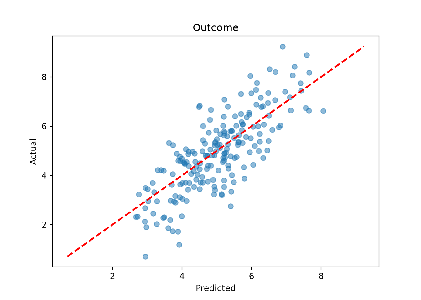

rmse = np.sqrt(np.mean(np.power(y_hat_test - y_test, 2)))
print(f"Test-set RMSE: {rmse:.2f}")

Test-set RMSE: 0.99

Compare true versus estimated treatment effects for each treatment entry

R

tau_hat_test <- predict(
  bcf_model,
  X = X_test,
  Z = Z_test,
  propensity = pi_test,
  terms = "cate",
  type = "mean"
)
plot(
  tau_test[, 1],
  tau_hat_test[, 1],
  xlab = "True tau",
  ylab = "Average estimated tau",
  main = "Treatment 1"
)
abline(0, 1, col = "black", lty = 3)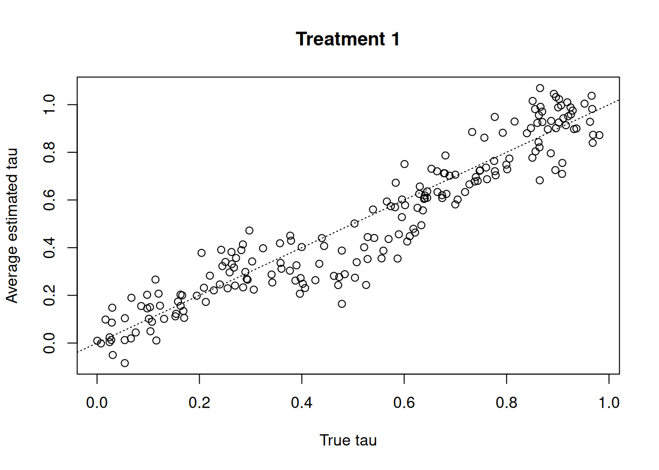

plot(
  tau_test[, 2],
  tau_hat_test[, 2],
  xlab = "True tau",
  ylab = "Average estimated tau",
  main = "Treatment 2"
)
abline(0, 1, col = "black", lty = 3)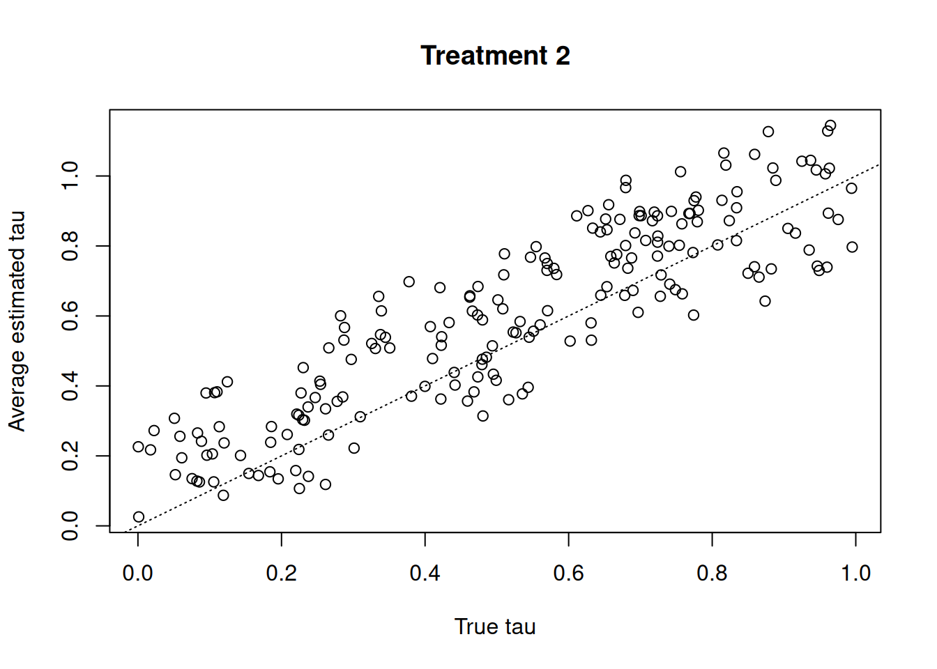

Python

tau_hat_test = bcf_model.predict(
    X=X_test, Z=Z_test, propensity=pi_test, terms="cate", type="mean"
)
treatment_idx = 0
lo, hi = (
    min((tau_hat_test[:, treatment_idx]).min(), (tau_test[:, treatment_idx]).min()),
    max((tau_hat_test[:, treatment_idx]).max(), (tau_test[:, treatment_idx]).max()),
)
plt.scatter(tau_test[:, treatment_idx], tau_hat_test[:, treatment_idx], alpha=0.5)
plt.plot([lo, hi], [lo, hi], color="red", linestyle="dashed", linewidth=2)
plt.xlabel("True tau")
plt.ylabel("Average estimated tau")
plt.title(f"Treatment {treatment_idx + 1}")
plt.show()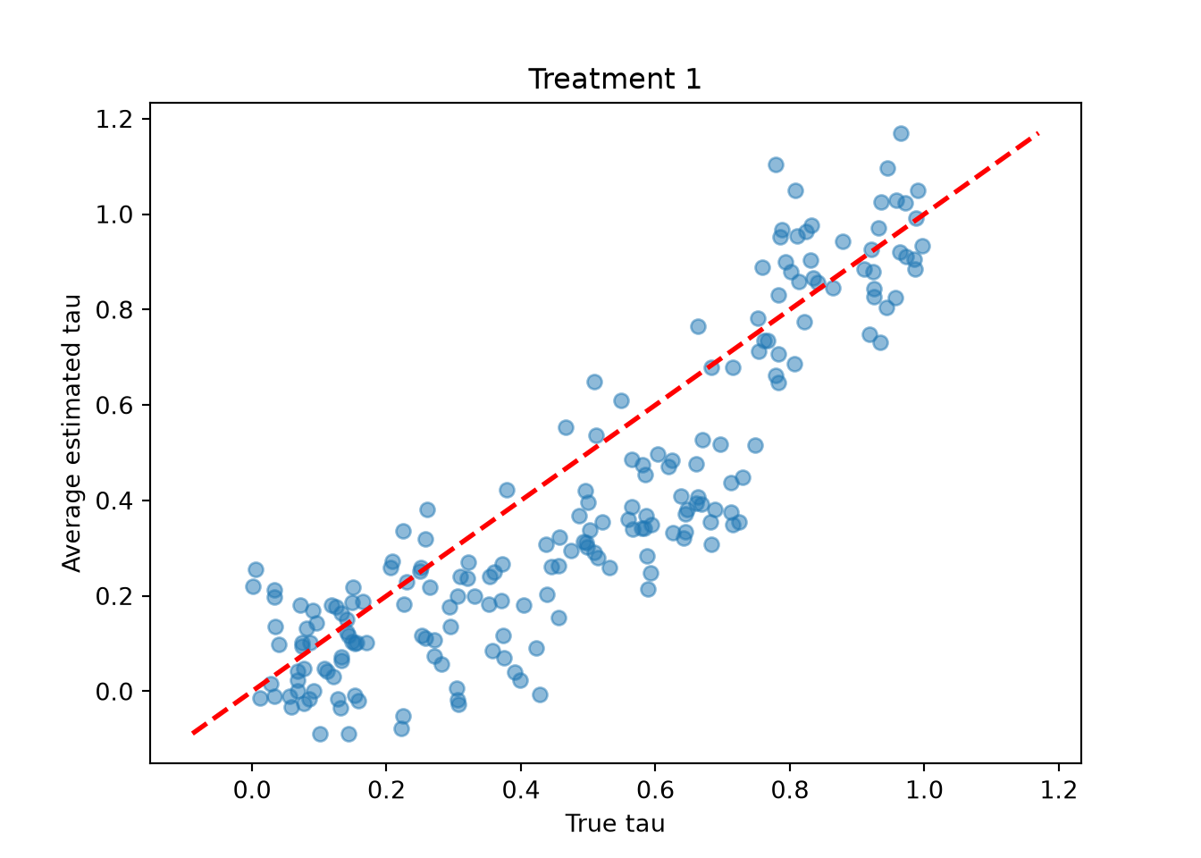

treatment_idx = 1
lo, hi = (
    min((tau_hat_test[:, treatment_idx]).min(), (tau_test[:, treatment_idx]).min()),
    max((tau_hat_test[:, treatment_idx]).max(), (tau_test[:, treatment_idx]).max()),
)
plt.scatter(tau_test[:, treatment_idx], tau_hat_test[:, treatment_idx], alpha=0.5)
plt.plot([lo, hi], [lo, hi], color="red", linestyle="dashed", linewidth=2)
plt.xlabel("True tau")
plt.ylabel("Average estimated tau")
plt.title(f"Treatment {treatment_idx + 1}")
plt.show()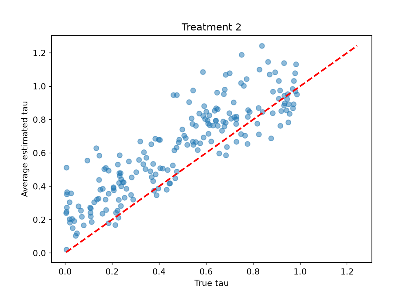

Now compare the true versus estimated treatment terms of the model (i.e. \(t_i = \sum_j(\tau_{i,j}(X) * Z_{i,j})\) where \(i\) indexes observations and \(j\) indexes treatments)

R

tau_hat_test <- predict(
  bcf_model,
  X = X_test,
  Z = Z_test,
  propensity = pi_test,
  terms = "cate",
  type = "posterior"
)
treatment_term_mcmc <- apply(tau_hat_test, 3, function(tau_s) {
  rowSums(tau_s * Z_test)
})
true_treatment_term <- rowSums(tau_test * Z_test)
plot(
  true_treatment_term,
  rowMeans(treatment_term_mcmc),
  xlab = "True treatment term",
  ylab = "Average estimated treatment term"
)
abline(0, 1, col = "black", lty = 3)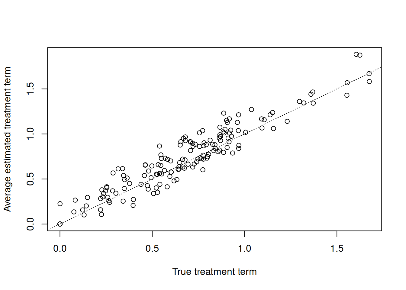

Python

tau_hat_test = bcf_model.predict(
    X=X_test, Z=Z_test, propensity=pi_test, terms="cate", type="posterior"
)
# tau_hat_test has shape (n, num_samples, treatment_dim), so the treatment
# dimension is summed over on axis 2
treatment_term_mcmc_test = np.multiply(
    np.atleast_3d(Z_test).swapaxes(1, 2), tau_hat_test
).sum(axis=2)
treatment_term_test = np.multiply(tau_test, Z_test).sum(axis=1)
treatment_term_hat_test = np.squeeze(treatment_term_mcmc_test).mean(
    axis=1, keepdims=True
)
lo, hi = (
    min((treatment_term_hat_test).min(), (treatment_term_test).min()),
    max((treatment_term_hat_test).max(), (treatment_term_test).max()),
)
plt.scatter(treatment_term_test, treatment_term_hat_test, alpha=0.5)
plt.plot([lo, hi], [lo, hi], color="red", linestyle="dashed", linewidth=2)
plt.xlabel("True value")
plt.ylabel("Average estimated value")
plt.title("Treatment Term")
plt.show()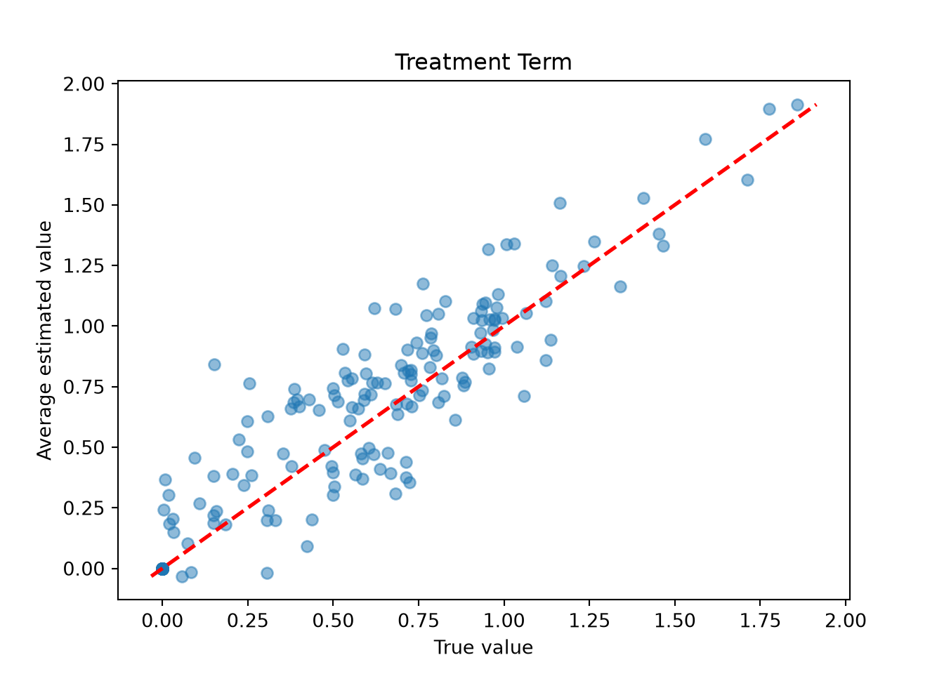

Compare true and predicted prognostic function values

R

mu_hat_test <- predict(
  bcf_model,
  X = X_test,
  Z = Z_test,
  propensity = pi_test,
  terms = "prognostic_function",
  type = "mean"
)
plot(
  mu_test,
  mu_hat_test,
  xlab = "True value",
  ylab = "Average estimated value",
  main = "Prognostic Function"
)
abline(0, 1, col = "black", lty = 3)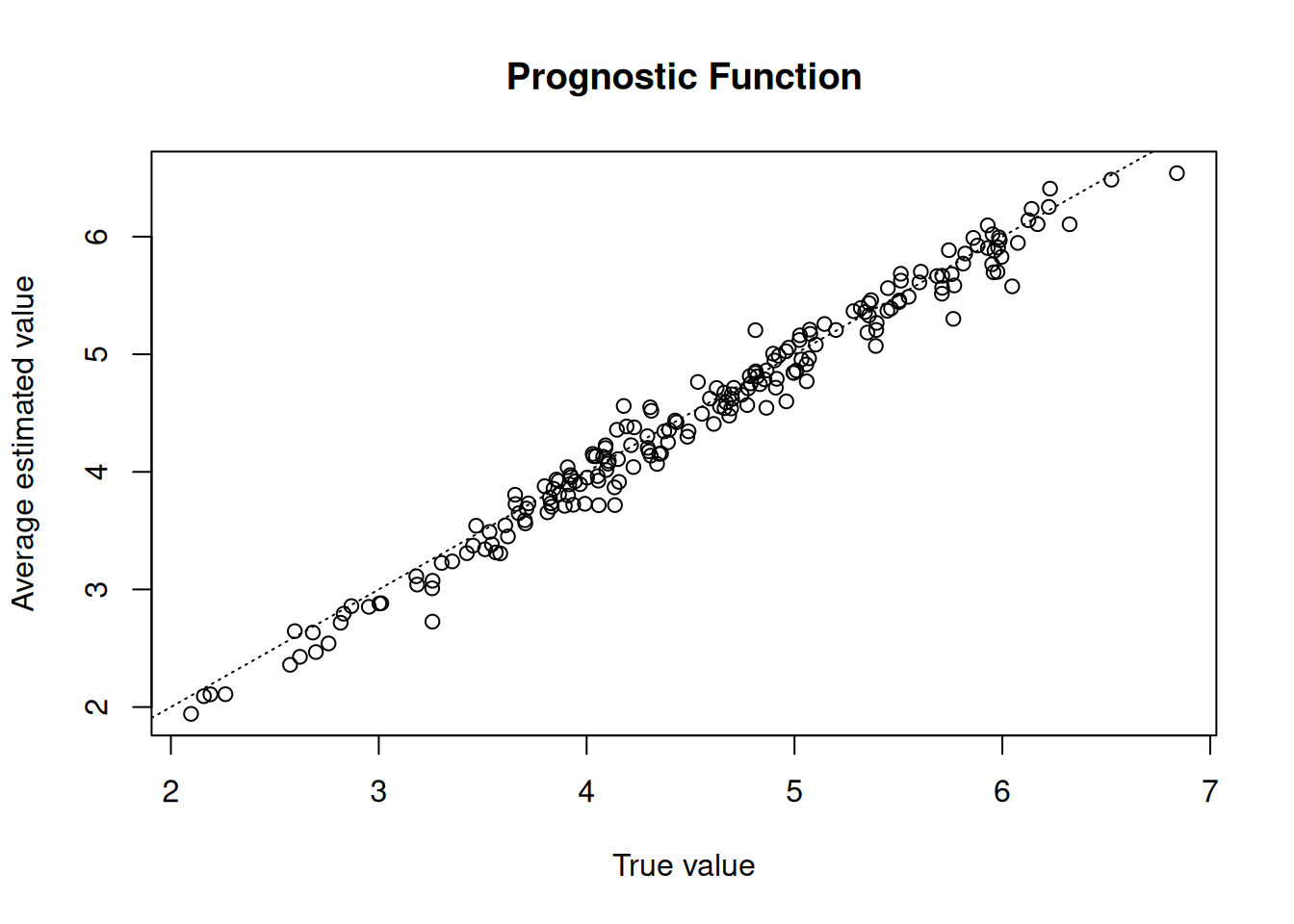

Python

mu_hat_test = bcf_model.predict(
    X=X_test, Z=Z_test, propensity=pi_test, terms="prognostic_function", type="mean"
)
lo, hi = (
    min((mu_hat_test).min(), (mu_test).min()),
    max((mu_hat_test).max(), (mu_test).max()),
)
plt.scatter(mu_hat_test, mu_test, alpha=0.5)
plt.plot([lo, hi], [lo, hi], color="red", linestyle="dashed", linewidth=2)
plt.xlabel("True value")
plt.ylabel("Average estimated value")
plt.title("Prognostic Function")
plt.show()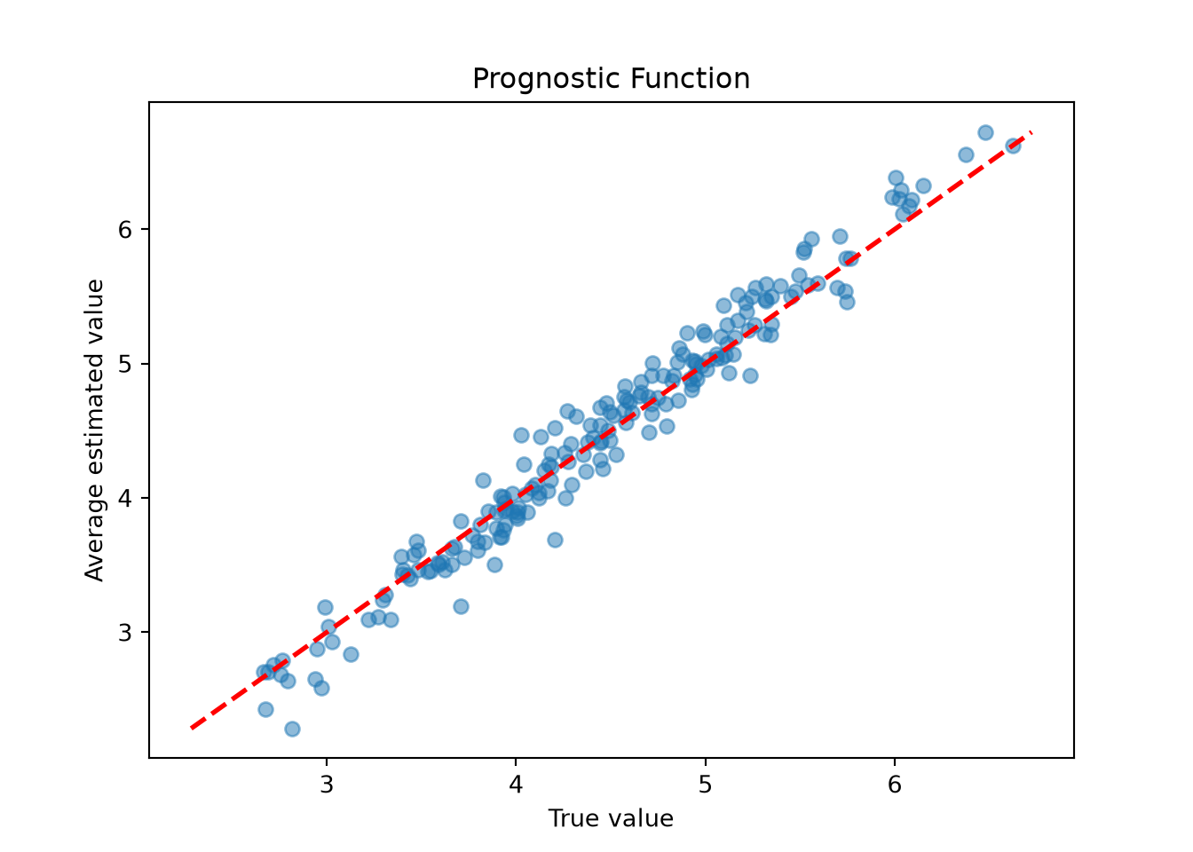

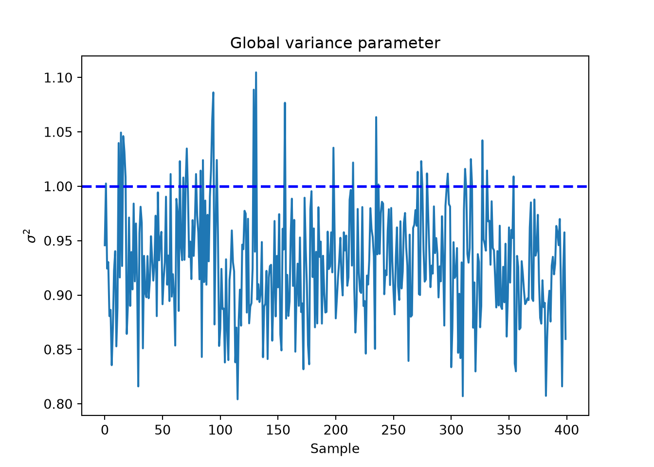
Finally, we inspect the traceplot of the global error variance, \(\sigma^2\)

R

sigma2_global_samples <- extractParameter(bcf_model, "sigma2_global")
plot(
  sigma2_global_samples,
  xlab = "Sample",
  ylab = expression(sigma^2)
)
abline(h = 1, lty = 3, lwd = 3, col = "blue")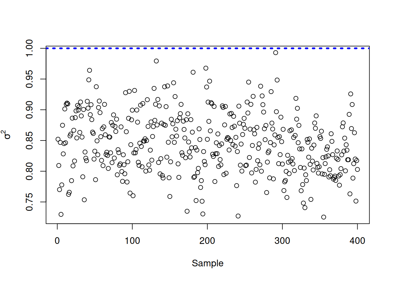

Python

global_var_samples = bcf_model.extract_parameter("sigma2_global")
plt.plot(global_var_samples)
plt.axhline(1, color="blue", linestyle="dashed", linewidth=2)
plt.xlabel("Sample")
plt.ylabel(r"$\sigma^2$")
plt.title("Global variance parameter")
plt.show()