Calibrating Leaf Node Scale Parameter Priors

This vignette demonstrates prior calibration approaches for the parametric components of stochastic tree ensembles (Chipman et al. (2010)).

Background

The “classic” BART model of Chipman et al. (2010)

\[\begin{equation*} \begin{aligned} y &= f(X) + \epsilon\\ f(X) &\sim \text{BART}\left(\alpha, \beta\right)\\ \epsilon &\sim \mathcal{N}\left(0,\sigma^2\right)\\ \sigma^2 &\sim \text{IG}\left(a,b\right) \end{aligned} \end{equation*}\]

is semiparametric, with a nonparametric tree ensemble \(f(X)\) and a homoskedastic error variance parameter \(\sigma^2\). Note that in Chipman et al. (2010), \(a\) and \(b\) are parameterized with \(a = \frac{\nu}{2}\) and \(b = \frac{\nu\lambda}{2}\).

Setting Priors on Variance Parameters in stochtree

By default, stochtree employs a Jeffreys’ prior for \(\sigma^2\) \[\begin{equation*} \begin{aligned} \sigma^2 &\propto \frac{1}{\sigma^2} \end{aligned} \end{equation*}\] which corresponds to an improper prior with \(a = 0\) and \(b = 0\).

We provide convenience functions for users wishing to set the \(\sigma^2\) prior as in Chipman et al. (2010). In this case, \(\nu\) is set by default to 3 and \(\lambda\) is calibrated as follows:

1. An “overestimate,” \(\hat{\sigma}^2\), of \(\sigma^2\) is obtained via simple linear regression of \(y\) on \(X\)
2. \(\lambda\) is chosen to ensure that \(p(\sigma^2 < \hat{\sigma}^2) = q\) for some value \(q\), typically set to a default value of 0.9.

Setup

Load the necessary packages

R

library(stochtree)

Python

import numpy as np
import matplotlib.pyplot as plt
from stochtree import BARTModel, calibrate_global_error_variance

Set a seed for reproducibility

R

random_seed <- 1234
set.seed(random_seed)

Python

random_seed = 1234
rng = np.random.default_rng(random_seed)

Data Generation

Generate data for a straightforward supervised learning problem

R

n <- 500
p <- 5
X <- matrix(runif(n*p), ncol = p)
f_XW <- (
    ((0 <= X[,1]) & (0.25 > X[,1])) * (-7.5) +
    ((0.25 <= X[,1]) & (0.5 > X[,1])) * (-2.5) +
    ((0.5 <= X[,1]) & (0.75 > X[,1])) * (2.5) +
    ((0.75 <= X[,1]) & (1 > X[,1])) * (7.5)
)
noise_sd <- 1
y <- f_XW + rnorm(n, 0, noise_sd)

Python

n = 500
p = 5
X = rng.uniform(size=(n, p))
f_XW = (
    ((X[:, 0] >= 0)    & (X[:, 0] < 0.25)) * (-7.5) +
    ((X[:, 0] >= 0.25) & (X[:, 0] < 0.5))  * (-2.5) +
    ((X[:, 0] >= 0.5)  & (X[:, 0] < 0.75)) * (2.5)  +
    ((X[:, 0] >= 0.75) & (X[:, 0] < 1.0))  * (7.5)
)
noise_sd = 1.0
y = f_XW + rng.normal(0, noise_sd, n)

Split into train and test set

R

test_set_pct <- 0.2
n_test <- round(test_set_pct*n)
n_train <- n - n_test
test_inds <- sort(sample(1:n, n_test, replace = FALSE))
train_inds <- (1:n)[!((1:n) %in% test_inds)]
X_test <- X[test_inds,]
X_train <- X[train_inds,]
y_test <- y[test_inds]
y_train <- y[train_inds]

Python

test_set_pct = 0.2
n_test = round(test_set_pct * n)
n_train = n - n_test
test_inds = rng.choice(n, n_test, replace=False)
train_inds = np.setdiff1d(np.arange(n), test_inds)
X_test = X[test_inds]
X_train = X[train_inds]
y_test = y[test_inds]
y_train = y[train_inds]

Model Sampling

First, we calibrate the scale parameter for the variance term as in Chipman et al (2010)

R

nu <- 3
lambda <- calibrateInverseGammaErrorVariance(y_train, X_train, nu = nu)

Python

nu = 3
lambda_ = calibrate_global_error_variance(X_train, y_train, nu=nu)

Then, we run a BART model with this variance parameterization

R

general_params <- list(sigma2_global_shape = nu/2, sigma2_global_scale = (nu*lambda)/2)
bart_model <- bart(X_train = X_train, y_train = y_train, X_test = X_test,
                   num_gfr = 0, num_burnin = 1000, num_mcmc = 100,
                   general_params = general_params)

Python

bart_model = BARTModel()
bart_model.sample(
    X_train=X_train, y_train=y_train, X_test=X_test,
    num_gfr=0, num_burnin=1000, num_mcmc=100,
    general_params={
        "num_threads": 1,
        "sigma2_global_shape": nu / 2,
        "sigma2_global_scale": (nu * lambda_) / 2,
    },
)

BARTModel run with mean forest, global error variance model, and mean forest leaf scale model
Outcome was modeled as gaussian with a constant leaf prior for the mean forest
Outcome was standardized
The sampler was run for 0 GFR iterations, with 1 chain of 1000 burn-in iterations and 100 MCMC iterations, retaining every iteration (i.e. no thinning)

Inspect the out-of-sample predictions of the model

R

plot(rowMeans(extractParameter(bart_model, "y_hat_test")), y_test, xlab = "predicted", ylab = "actual")
abline(0,1,col="red",lty=3,lwd=3)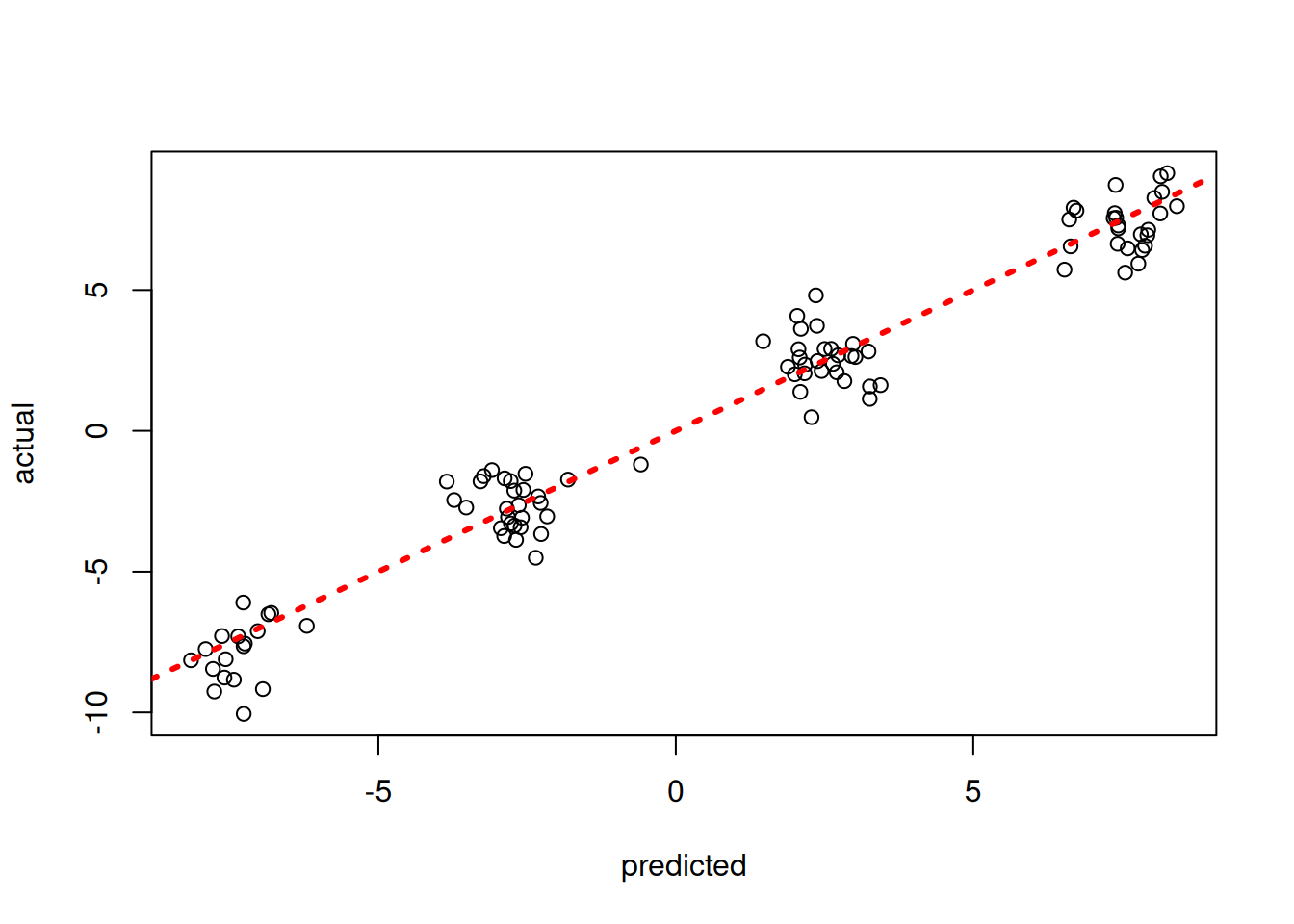

Python

pred_mean = bart_model.y_hat_test.mean(axis=1)

<string>:1: DeprecationWarning: `BARTModel.y_hat_test` is deprecated and will be removed in a future release. The sampled values are owned by `model.samples`; use `model.extract_parameter("y_hat_test")` instead.

lo = min(pred_mean.min(), y_test.min())
hi = max(pred_mean.max(), y_test.max())
plt.scatter(pred_mean, y_test, alpha=0.5)
plt.plot([lo, hi], [lo, hi], color="red", linestyle="dashed", linewidth=2)
plt.xlabel("Predicted")
plt.ylabel("Actual")
plt.show()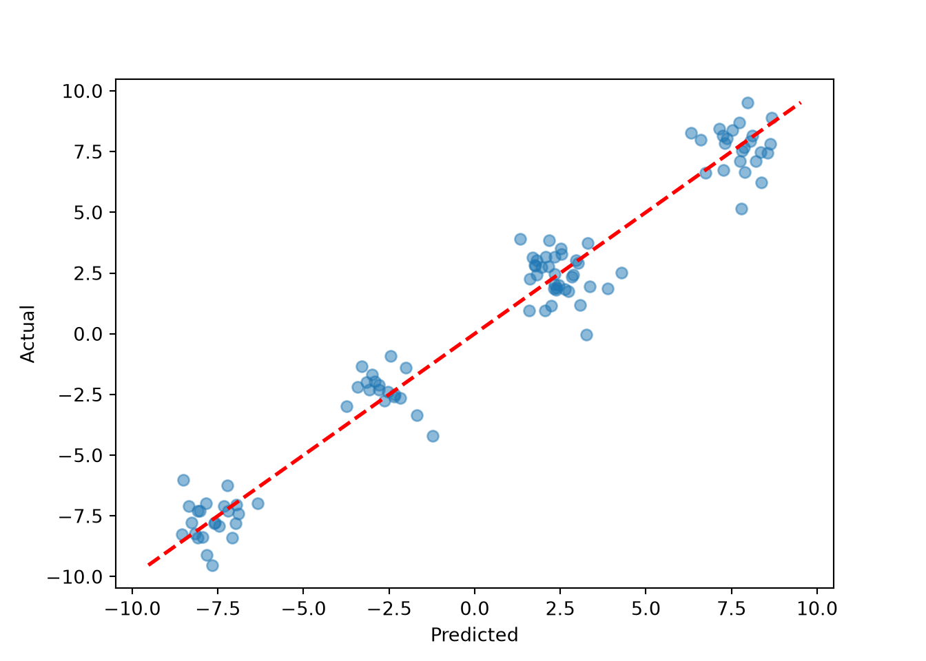

Inspect the posterior samples of \(\sigma^2\)

R

plot(extractParameter(bart_model, "sigma2_global"), ylab = "sigma^2", xlab = "iteration")
abline(h = noise_sd^2, col = "red", lty = 3, lwd = 3)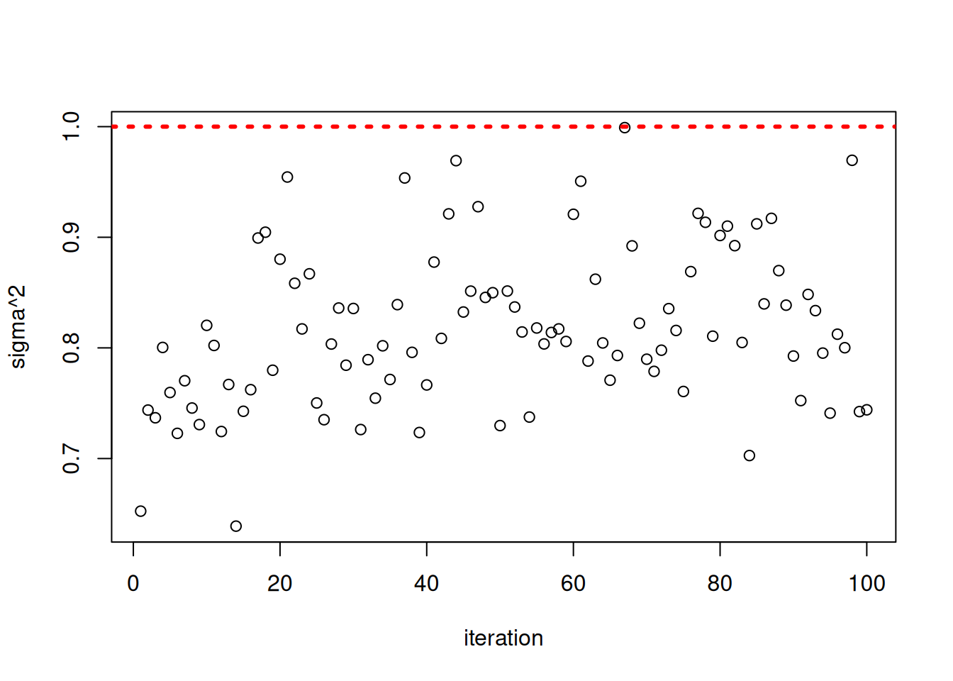

Python

plt.plot(bart_model.global_var_samples)
plt.xlabel("Iteration")
plt.ylabel(r"$\sigma^2$")
plt.axhline(noise_sd**2, color="red", linestyle="dashed", linewidth=2)
plt.show()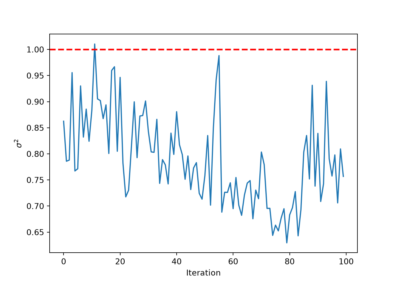

References

Chipman, Hugh A., Edward I. George, and Robert E. McCulloch. 2010. “BART: Bayesian additive regression trees.” The Annals of Applied Statistics 4 (1): 266–98. https://doi.org/10.1214/09-AOAS285.