Bayesian Supervised Learning in StochTree
Source:vignettes/BayesianSupervisedLearning.Rmd
BayesianSupervisedLearning.RmdThis vignette demonstrates how to use the bart()
function for Bayesian supervised learning (Chipman, George, and McCulloch (2010)). To
begin, we load the stochtree package.
Demo 1: Step Function
Simulation
Here, we generate data from a simple step function.
# Generate the data
n <- 500
p_x <- 10
snr <- 3
X <- matrix(runif(n * p_x), ncol = p_x)
f_XW <- (((0 <= X[, 1]) & (0.25 > X[, 1])) *
  (-7.5) +
  ((0.25 <= X[, 1]) & (0.5 > X[, 1])) * (-2.5) +
  ((0.5 <= X[, 1]) & (0.75 > X[, 1])) * (2.5) +
  ((0.75 <= X[, 1]) & (1 > X[, 1])) * (7.5))
noise_sd <- sd(f_XW) / snr
y <- f_XW + rnorm(n, 0, 1) * noise_sd

# Split data into test and train sets
test_set_pct <- 0.2
n_test <- round(test_set_pct * n)
n_train <- n - n_test
test_inds <- sort(sample(1:n, n_test, replace = FALSE))
train_inds <- (1:n)[!((1:n) %in% test_inds)]
X_test <- as.data.frame(X[test_inds, ])
X_train <- as.data.frame(X[train_inds, ])
y_test <- y[test_inds]
y_train <- y[train_inds]
Sampling and Analysis
Warmstart
We first sample from an ensemble model of
using “warm-start” initialization samples (He and
Hahn (2023)). This is the default in stochtree.
num_gfr <- 10
num_burnin <- 0
num_mcmc <- 100
num_samples <- num_gfr + num_burnin + num_mcmc
general_params <- list(sample_sigma2_global = T)
mean_forest_params <- list(sample_sigma2_leaf = T, num_trees = 100)
bart_model_warmstart <- stochtree::bart(
  X_train = X_train,
  y_train = y_train,
  X_test = X_test,
  num_gfr = num_gfr,
  num_burnin = num_burnin,
  num_mcmc = num_mcmc,
  general_params = general_params,
  mean_forest_params = mean_forest_params
)
Inspect the MCMC samples
plot(bart_model_warmstart$sigma2_global_samples, ylab = "sigma^2")
abline(h = noise_sd^2, col = "red", lty = 2, lwd = 2.5)
plot(
  rowMeans(bart_model_warmstart$y_hat_test),
  y_test,
  pch = 16,
  cex = 0.75,
  xlab = "pred",
  ylab = "actual"
)
abline(0, 1, col = "red", lty = 2, lwd = 2.5)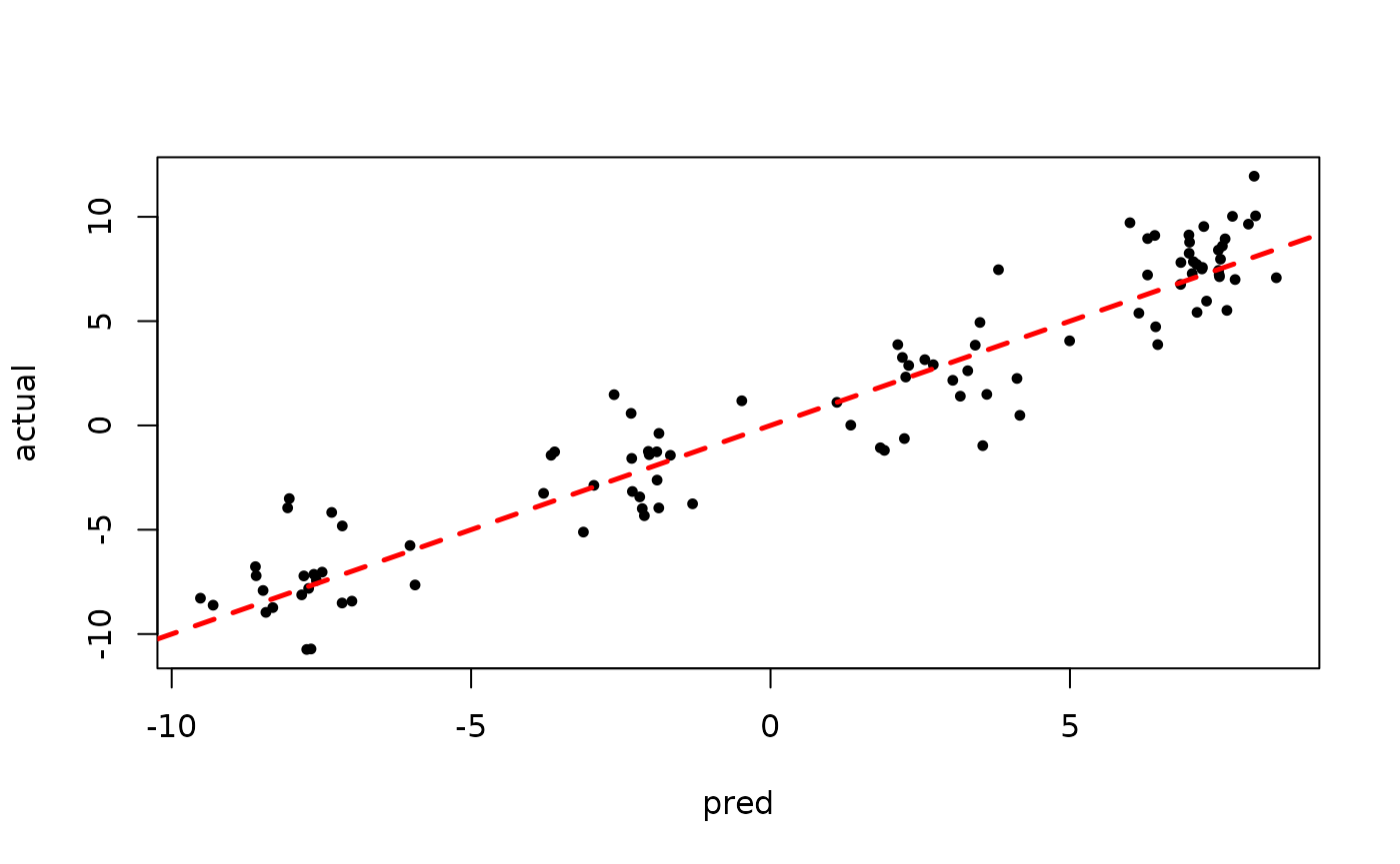
BART MCMC without Warmstart
Next, we sample from this ensemble model without any warm-start initialization.
num_gfr <- 0
num_burnin <- 100
num_mcmc <- 100
num_samples <- num_gfr + num_burnin + num_mcmc
general_params <- list(sample_sigma2_global = T)
mean_forest_params <- list(sample_sigma2_leaf = T, num_trees = 100)
bart_model_root <- stochtree::bart(
  X_train = X_train,
  y_train = y_train,
  X_test = X_test,
  num_gfr = num_gfr,
  num_burnin = num_burnin,
  num_mcmc = num_mcmc,
  general_params = general_params,
  mean_forest_params = mean_forest_params
)
Inspect the MCMC samples
plot(bart_model_root$sigma2_global_samples, ylab = "sigma^2")
abline(h = noise_sd^2, col = "red", lty = 2, lwd = 2.5)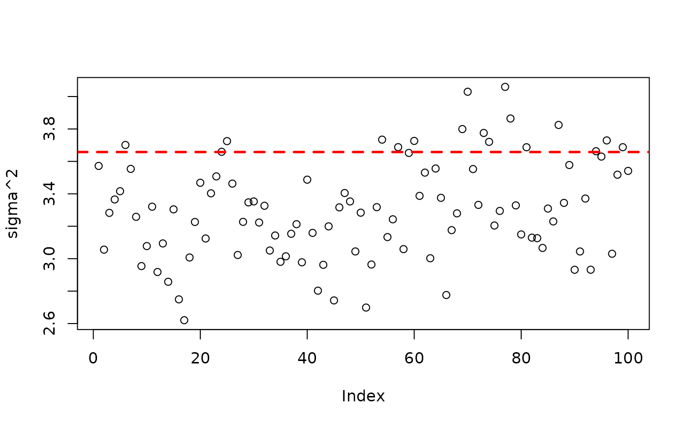
plot(
  rowMeans(bart_model_root$y_hat_test),
  y_test,
  pch = 16,
  cex = 0.75,
  xlab = "pred",
  ylab = "actual"
)
abline(0, 1, col = "red", lty = 2, lwd = 2.5)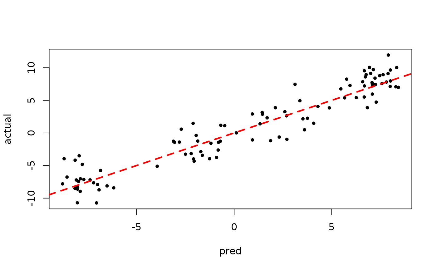
Demo 2: Partitioned Linear Model
Simulation
Here, we generate data from a simple partitioned linear model.
# Generate the data
n <- 500
p_x <- 10
p_w <- 1
snr <- 3
X <- matrix(runif(n * p_x), ncol = p_x)
leaf_basis <- matrix(runif(n * p_w), ncol = p_w)
f_XW <- (((0 <= X[, 1]) & (0.25 > X[, 1])) *
  (-7.5 * leaf_basis[, 1]) +
  ((0.25 <= X[, 1]) & (0.5 > X[, 1])) * (-2.5 * leaf_basis[, 1]) +
  ((0.5 <= X[, 1]) & (0.75 > X[, 1])) * (2.5 * leaf_basis[, 1]) +
  ((0.75 <= X[, 1]) & (1 > X[, 1])) * (7.5 * leaf_basis[, 1]))
noise_sd <- sd(f_XW) / snr
y <- f_XW + rnorm(n, 0, 1) * noise_sd

# Split data into test and train sets
test_set_pct <- 0.2
n_test <- round(test_set_pct * n)
n_train <- n - n_test
test_inds <- sort(sample(1:n, n_test, replace = FALSE))
train_inds <- (1:n)[!((1:n) %in% test_inds)]
X_test <- as.data.frame(X[test_inds, ])
X_train <- as.data.frame(X[train_inds, ])
leaf_basis_test <- leaf_basis[test_inds, ]
leaf_basis_train <- leaf_basis[train_inds, ]
y_test <- y[test_inds]
y_train <- y[train_inds]
Sampling and Analysis
Warmstart
We first sample from an ensemble model of
using “warm-start” initialization samples (He and
Hahn (2023)). This is the default in stochtree.
num_gfr <- 10
num_burnin <- 0
num_mcmc <- 100
num_samples <- num_gfr + num_burnin + num_mcmc
general_params <- list(sample_sigma2_global = T)
mean_forest_params <- list(sample_sigma2_leaf = T, num_trees = 100)
bart_model_warmstart <- stochtree::bart(
  X_train = X_train,
  leaf_basis_train = leaf_basis_train,
  y_train = y_train,
  X_test = X_test,
  leaf_basis_test = leaf_basis_test,
  num_gfr = num_gfr,
  num_burnin = num_burnin,
  num_mcmc = num_mcmc,
  general_params = general_params,
  mean_forest_params = mean_forest_params
)
Inspect the MCMC samples
plot(bart_model_warmstart$sigma2_global_samples, ylab = "sigma^2")
abline(h = noise_sd^2, col = "red", lty = 2, lwd = 2.5)
plot(
  rowMeans(bart_model_warmstart$y_hat_test),
  y_test,
  pch = 16,
  cex = 0.75,
  xlab = "pred",
  ylab = "actual"
)
abline(0, 1, col = "red", lty = 2, lwd = 2.5)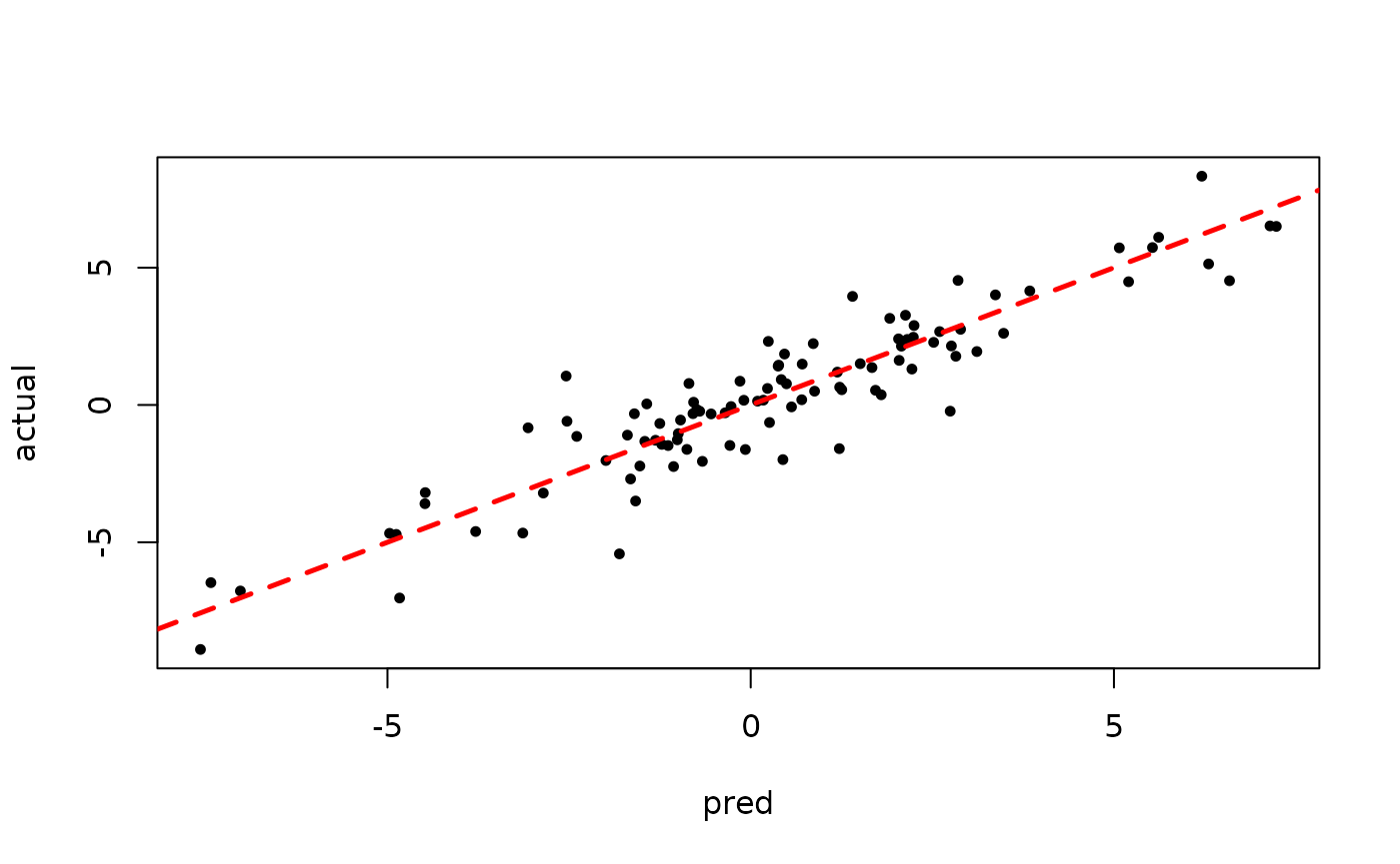
BART MCMC without Warmstart
Next, we sample from this ensemble model without any warm-start initialization.
num_gfr <- 0
num_burnin <- 100
num_mcmc <- 100
num_samples <- num_gfr + num_burnin + num_mcmc
general_params <- list(sample_sigma2_global = T)
mean_forest_params <- list(sample_sigma2_leaf = T, num_trees = 100)
bart_model_root <- stochtree::bart(
  X_train = X_train,
  leaf_basis_train = leaf_basis_train,
  y_train = y_train,
  X_test = X_test,
  leaf_basis_test = leaf_basis_test,
  num_gfr = num_gfr,
  num_burnin = num_burnin,
  num_mcmc = num_mcmc,
  general_params = general_params,
  mean_forest_params = mean_forest_params
)
Inspect the BART samples after burnin.
plot(bart_model_root$sigma2_global_samples, ylab = "sigma^2")
abline(h = noise_sd^2, col = "red", lty = 2, lwd = 2.5)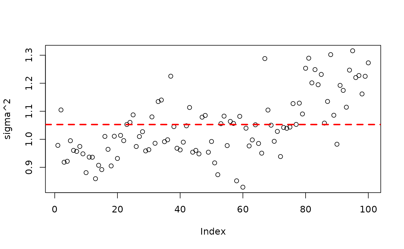
plot(
  rowMeans(bart_model_root$y_hat_test),
  y_test,
  pch = 16,
  cex = 0.75,
  xlab = "pred",
  ylab = "actual"
)
abline(0, 1, col = "red", lty = 2, lwd = 2.5)
Demo 3: Partitioned Linear Model with Random Effects
Simulation
Here, we generate data from a simple partitioned linear model with an additive random effect structure.
# Generate the data
n <- 500
p_x <- 10
p_w <- 1
snr <- 3
X <- matrix(runif(n * p_x), ncol = p_x)
leaf_basis <- matrix(runif(n * p_w), ncol = p_w)
rfx_group_ids <- rep(c(1, 2), n %/% 2)
rfx_coefs <- matrix(c(-5, -3, 5, 3), nrow = 2, byrow = TRUE)
rfx_basis <- cbind(1, runif(n, -1, 1))
f_XW <- (((0 <= X[, 1]) & (0.25 > X[, 1])) *
  (-7.5 * leaf_basis[, 1]) +
  ((0.25 <= X[, 1]) & (0.5 > X[, 1])) * (-2.5 * leaf_basis[, 1]) +
  ((0.5 <= X[, 1]) & (0.75 > X[, 1])) * (2.5 * leaf_basis[, 1]) +
  ((0.75 <= X[, 1]) & (1 > X[, 1])) * (7.5 * leaf_basis[, 1]))
rfx_term <- rowSums(rfx_coefs[rfx_group_ids, ] * rfx_basis)
noise_sd <- sd(f_XW) / snr
y <- f_XW + rfx_term + rnorm(n, 0, 1) * noise_sd

# Split data into test and train sets
test_set_pct <- 0.2
n_test <- round(test_set_pct * n)
n_train <- n - n_test
test_inds <- sort(sample(1:n, n_test, replace = FALSE))
train_inds <- (1:n)[!((1:n) %in% test_inds)]
X_test <- as.data.frame(X[test_inds, ])
X_train <- as.data.frame(X[train_inds, ])
leaf_basis_test <- leaf_basis[test_inds, ]
leaf_basis_train <- leaf_basis[train_inds, ]
y_test <- y[test_inds]
y_train <- y[train_inds]
rfx_group_ids_test <- rfx_group_ids[test_inds]
rfx_group_ids_train <- rfx_group_ids[train_inds]
rfx_basis_test <- rfx_basis[test_inds, ]
rfx_basis_train <- rfx_basis[train_inds, ]
Sampling and Analysis
Warmstart
We first sample from an ensemble model of
using “warm-start” initialization samples (He and
Hahn (2023)). This is the default in stochtree.
num_gfr <- 10
num_burnin <- 0
num_mcmc <- 100
num_samples <- num_gfr + num_burnin + num_mcmc
general_params <- list(sample_sigma2_global = T)
mean_forest_params <- list(sample_sigma2_leaf = T, num_trees = 100)
bart_model_warmstart <- stochtree::bart(
  X_train = X_train,
  leaf_basis_train = leaf_basis_train,
  y_train = y_train,
  rfx_group_ids_train = rfx_group_ids_train,
  rfx_basis_train = rfx_basis_train,
  X_test = X_test,
  leaf_basis_test = leaf_basis_test,
  rfx_group_ids_test = rfx_group_ids_test,
  rfx_basis_test = rfx_basis_test,
  num_gfr = num_gfr,
  num_burnin = num_burnin,
  num_mcmc = num_mcmc,
  general_params = general_params,
  mean_forest_params = mean_forest_params
)
Inspect the MCMC samples
plot(bart_model_warmstart$sigma2_global_samples, ylab = "sigma^2")
abline(h = noise_sd^2, col = "red", lty = 2, lwd = 2.5)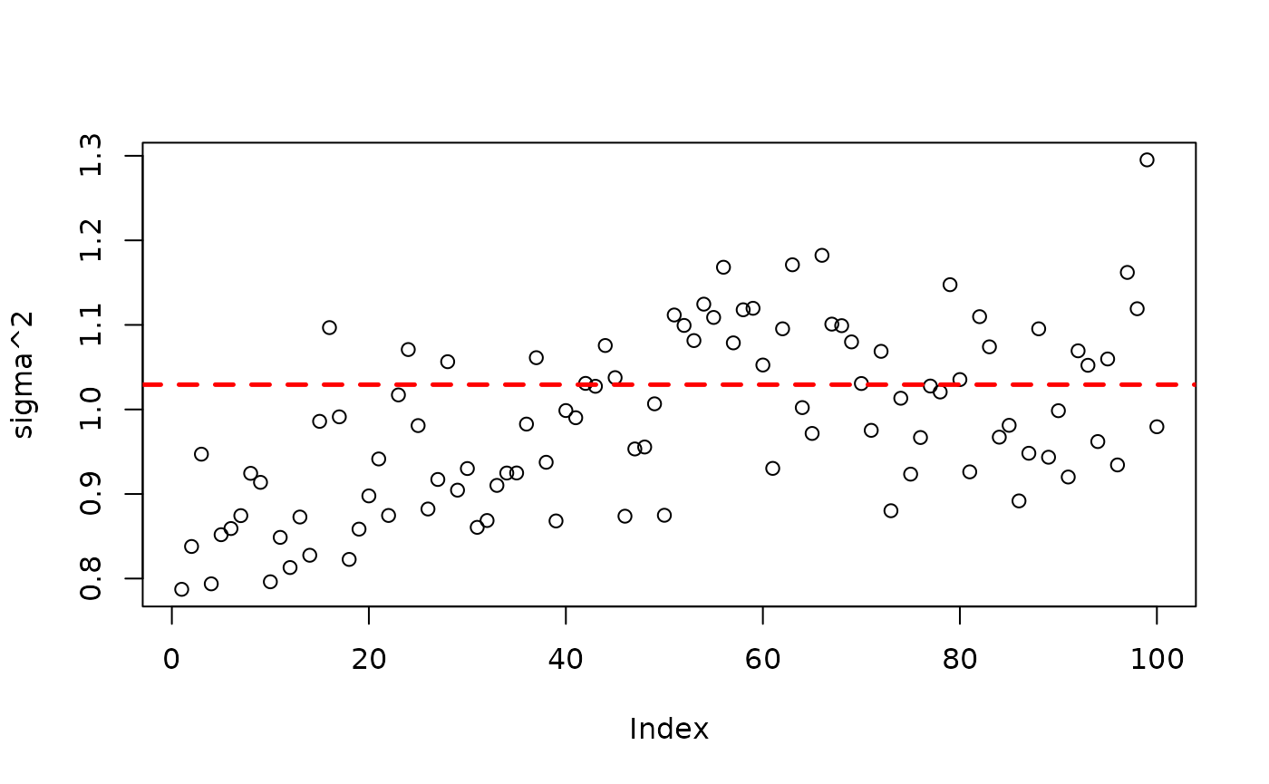
plot(
  rowMeans(bart_model_warmstart$y_hat_test),
  y_test,
  pch = 16,
  cex = 0.75,
  xlab = "pred",
  ylab = "actual"
)
abline(0, 1, col = "red", lty = 2, lwd = 2.5)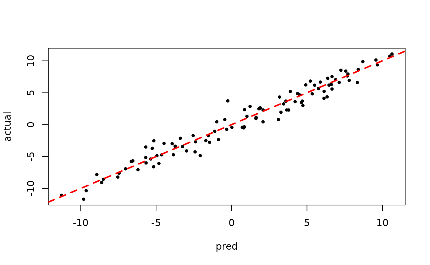
BART MCMC without Warmstart
Next, we sample from this ensemble model without any warm-start initialization.
num_gfr <- 0
num_burnin <- 100
num_mcmc <- 100
num_samples <- num_gfr + num_burnin + num_mcmc
general_params <- list(sample_sigma2_global = T)
mean_forest_params <- list(sample_sigma2_leaf = T, num_trees = 100)
bart_model_root <- stochtree::bart(
  X_train = X_train,
  leaf_basis_train = leaf_basis_train,
  y_train = y_train,
  rfx_group_ids_train = rfx_group_ids_train,
  rfx_basis_train = rfx_basis_train,
  X_test = X_test,
  leaf_basis_test = leaf_basis_test,
  rfx_group_ids_test = rfx_group_ids_test,
  rfx_basis_test = rfx_basis_test,
  num_gfr = num_gfr,
  num_burnin = num_burnin,
  num_mcmc = num_mcmc,
  general_params = general_params,
  mean_forest_params = mean_forest_params
)
Inspect the MCMC samples
plot(bart_model_root$sigma2_global_samples, ylab = "sigma^2")
abline(h = noise_sd^2, col = "red", lty = 2, lwd = 2.5)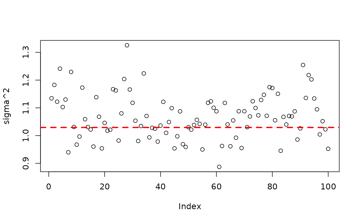
plot(
  rowMeans(bart_model_root$y_hat_test),
  y_test,
  pch = 16,
  cex = 0.75,
  xlab = "pred",
  ylab = "actual"
)
abline(0, 1, col = "red", lty = 2, lwd = 2.5)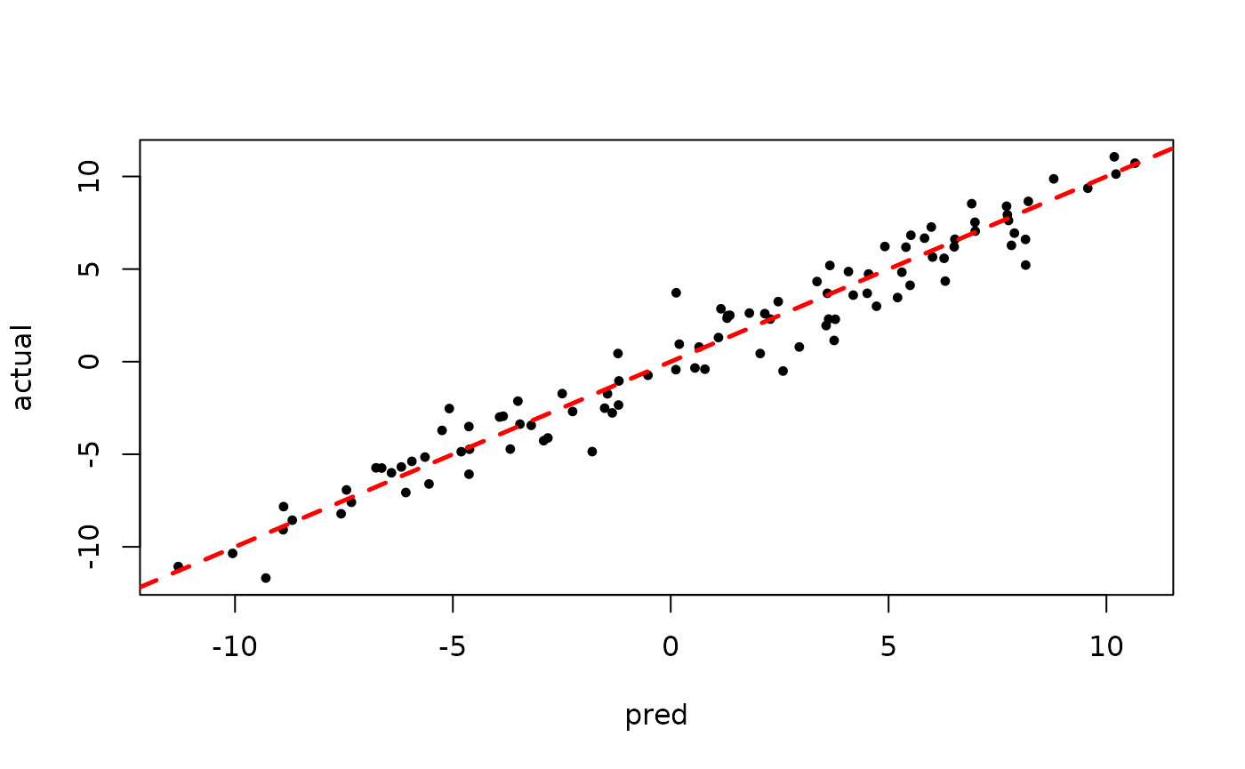
Demo 4: Partitioned Linear Model with Probit Outcome Model
Simulation
Here, we generate data from a simple partitioned linear model.
# Generate the data
n <- 1000
p_x <- 100
X <- matrix(runif(n * p_x), ncol = p_x)
f_X <- (((0 <= X[, 1]) & (0.25 > X[, 1])) *
  (-7.5 * X[, 2]) +
  ((0.25 <= X[, 1]) & (0.5 > X[, 1])) * (-2.5 * X[, 2]) +
  ((0.5 <= X[, 1]) & (0.75 > X[, 1])) * (2.5 * X[, 2]) +
  ((0.75 <= X[, 1]) & (1 > X[, 1])) * (7.5 * X[, 2]))
z <- f_X + rnorm(n, 0, 1)
y <- (z > 0) * 1.0

# Split data into test and train sets
test_set_pct <- 0.5
n_test <- round(test_set_pct * n)
n_train <- n - n_test
test_inds <- sort(sample(1:n, n_test, replace = FALSE))
train_inds <- (1:n)[!((1:n) %in% test_inds)]
X_test <- as.data.frame(X[test_inds, ])
X_train <- as.data.frame(X[train_inds, ])
z_test <- z[test_inds]
z_train <- z[train_inds]
y_test <- y[test_inds]
y_train <- y[train_inds]
Sampling and Analysis
Warmstart
We first sample from an ensemble model of
using “warm-start” initialization samples (He and
Hahn (2023)). This is the default in stochtree.
num_gfr <- 10
num_burnin <- 0
num_mcmc <- 100
num_samples <- num_gfr + num_burnin + num_mcmc
general_params <- list(
  sample_sigma2_global = F,
  outcome_model = OutcomeModel(outcome = "binary", link = "probit")
)
mean_forest_params <- list(sample_sigma2_leaf = F, num_trees = 100)
bart_model_warmstart <- stochtree::bart(
  X_train = X_train,
  y_train = y_train,
  X_test = X_test,
  num_gfr = num_gfr,
  num_burnin = num_burnin,
  num_mcmc = num_mcmc,
  general_params = general_params,
  mean_forest_params = mean_forest_params
)
Since we’ve simulated this data, we can compare the true latent continuous outcome variable to the probit-scale predictions for a test set.
plot(
  rowMeans(bart_model_warmstart$y_hat_test),
  z_test,
  pch = 16,
  cex = 0.75,
  xlab = "pred",
  ylab = "actual"
)
abline(0, 1, col = "red", lty = 2, lwd = 2.5)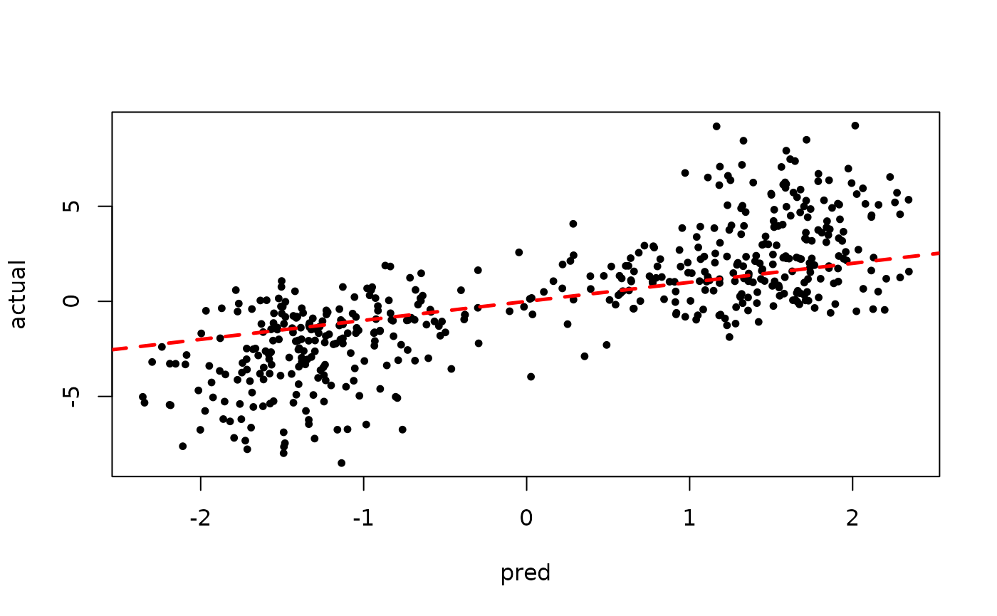
On non-simulated datasets, the first thing we would evaluate is the prediction accuracy.
We can also compute the ROC curve for every posterior sample, as well as the ROC of the posterior mean.
num_thresholds <- 1000
thresholds <- seq(0.001, 0.999, length.out = num_thresholds)
tpr_mean <- rep(NA, num_thresholds)
fpr_mean <- rep(NA, num_thresholds)
tpr_samples <- matrix(NA, num_thresholds, num_mcmc)
fpr_samples <- matrix(NA, num_thresholds, num_mcmc)
yhat_samples <- bart_model_warmstart$y_hat_test
yhat_mean <- rowMeans(yhat_samples)
for (i in 1:num_thresholds) {
  is_above_threshold_samples <- yhat_samples > qnorm(thresholds[i])
  is_above_threshold_mean <- yhat_mean > qnorm(thresholds[i])
  n_positive <- sum(y_test)
  n_negative <- sum(y_test == 0)
  y_above_threshold_mean <- y_test[is_above_threshold_mean]
  tpr_mean[i] <- sum(y_above_threshold_mean) / n_positive
  fpr_mean[i] <- sum(y_above_threshold_mean == 0) / n_negative
  for (j in 1:num_mcmc) {
    y_above_threshold <- y_test[is_above_threshold_samples[, j]]
    tpr_samples[i, j] <- sum(y_above_threshold) / n_positive
    fpr_samples[i, j] <- sum(y_above_threshold == 0) / n_negative
  }
}

for (i in 1:num_mcmc) {
  if (i == 1) {
    plot(
      fpr_samples[, i],
      tpr_samples[, i],
      type = "line",
      col = "blue",
      lwd = 1,
      lty = 1,
      xlab = "False positive rate",
      ylab = "True positive rate"
    )
  } else {
    lines(fpr_samples[, i], tpr_samples[, i], col = "blue", lwd = 1, lty = 1)
  }
}
#> Warning in plot.xy(xy, type, ...): plot type 'line' will be truncated to first
#> character
lines(fpr_mean, tpr_mean, col = "black", lwd = 3, lty = 3)
Note that the nonlinearity of the ROC function means that the ROC curve of the posterior mean could sit above most of the individual posterior sample ROC curves (which would not be the case if we had simply taken the mean of the ROC curves).
BART MCMC without Warmstart
Next, we sample from this ensemble model without any warm-start initialization.
num_gfr <- 0
num_burnin <- 100
num_mcmc <- 100
num_samples <- num_gfr + num_burnin + num_mcmc
general_params <- list(
  sample_sigma2_global = F,
  outcome_model = OutcomeModel(outcome = "binary", link = "probit")
)
mean_forest_params <- list(sample_sigma2_leaf = F, num_trees = 100)
bart_model_root <- stochtree::bart(
  X_train = X_train,
  y_train = y_train,
  X_test = X_test,
  num_gfr = num_gfr,
  num_burnin = num_burnin,
  num_mcmc = num_mcmc,
  general_params = general_params,
  mean_forest_params = mean_forest_params
)
Since we’ve simulated this data, we can compare the true latent continuous outcome variable to the probit-scale predictions for a test set.
plot(
  rowMeans(bart_model_root$y_hat_test),
  z_test,
  pch = 16,
  cex = 0.75,
  xlab = "pred",
  ylab = "actual"
)
abline(0, 1, col = "red", lty = 2, lwd = 2.5)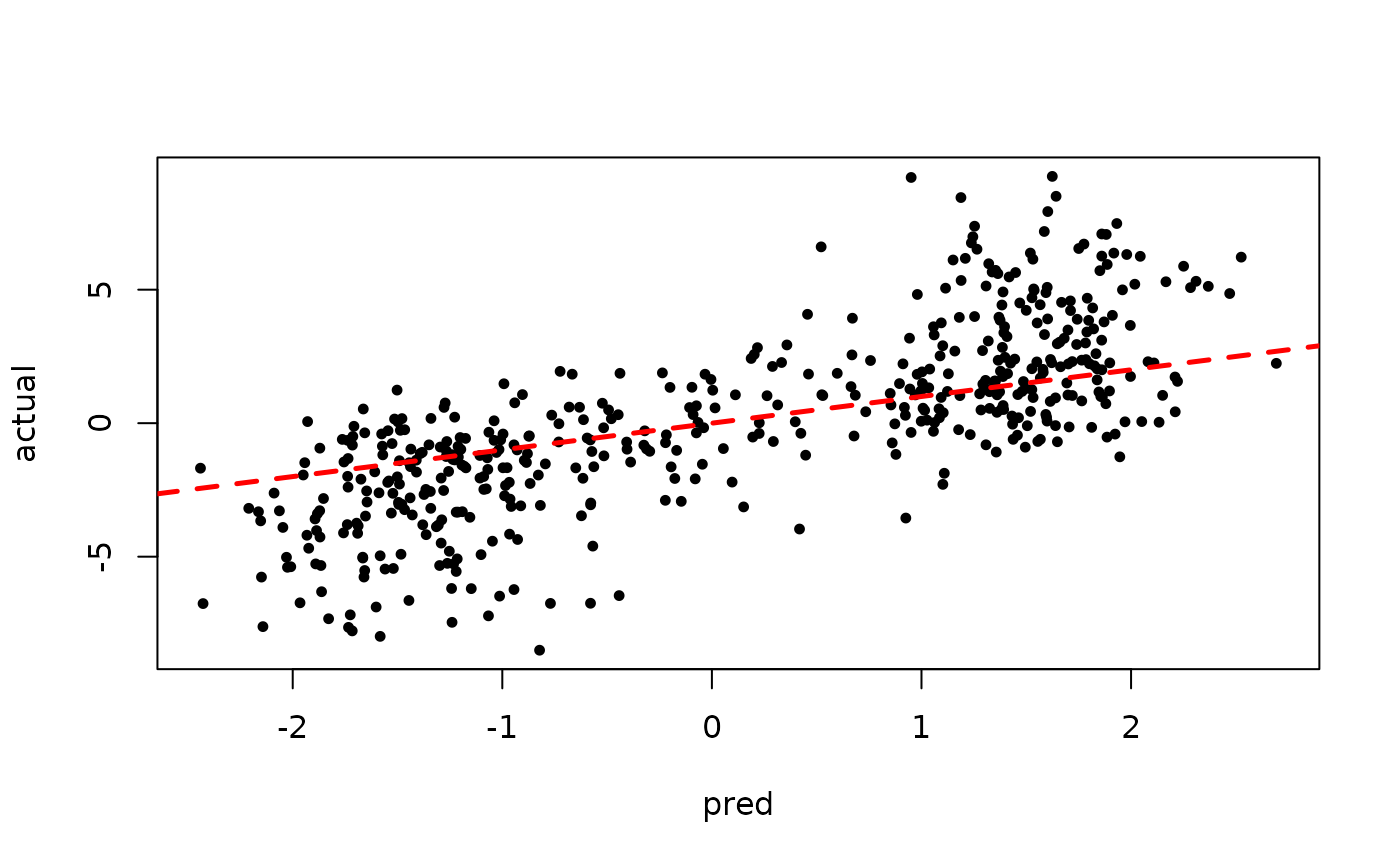
On non-simulated datasets, the first thing we would evaluate is the prediction accuracy.
We can also compute the ROC curve for every posterior sample, as well as the ROC of the posterior mean.
num_thresholds <- 1000
thresholds <- seq(0.001, 0.999, length.out = num_thresholds)
tpr_mean <- rep(NA, num_thresholds)
fpr_mean <- rep(NA, num_thresholds)
tpr_samples <- matrix(NA, num_thresholds, num_mcmc)
fpr_samples <- matrix(NA, num_thresholds, num_mcmc)
yhat_samples <- bart_model_root$y_hat_test
yhat_mean <- rowMeans(yhat_samples)
for (i in 1:num_thresholds) {
  is_above_threshold_samples <- yhat_samples > qnorm(thresholds[i])
  is_above_threshold_mean <- yhat_mean > qnorm(thresholds[i])
  n_positive <- sum(y_test)
  n_negative <- sum(y_test == 0)
  y_above_threshold_mean <- y_test[is_above_threshold_mean]
  tpr_mean[i] <- sum(y_above_threshold_mean) / n_positive
  fpr_mean[i] <- sum(y_above_threshold_mean == 0) / n_negative
  for (j in 1:num_mcmc) {
    y_above_threshold <- y_test[is_above_threshold_samples[, j]]
    tpr_samples[i, j] <- sum(y_above_threshold) / n_positive
    fpr_samples[i, j] <- sum(y_above_threshold == 0) / n_negative
  }
}

for (i in 1:num_mcmc) {
  if (i == 1) {
    plot(
      fpr_samples[, i],
      tpr_samples[, i],
      type = "line",
      col = "blue",
      lwd = 1,
      lty = 1,
      xlab = "False positive rate",
      ylab = "True positive rate"
    )
  } else {
    lines(fpr_samples[, i], tpr_samples[, i], col = "blue", lwd = 1, lty = 1)
  }
}
#> Warning in plot.xy(xy, type, ...): plot type 'line' will be truncated to first
#> character
lines(fpr_mean, tpr_mean, col = "black", lwd = 3, lty = 3)