Running Multiple Chains (Sequentially or in Parallel) in StochTree

Motivation

Mixing of an MCMC sampler is a perennial concern for complex Bayesian models. BART and BCF are no exception. On common way to address such concerns is to run multiple independent “chains” of an MCMC sampler, so that if each chain gets stuck in a different region of the posterior, their combined samples attain better coverage of the full posterior.

This idea works with the classic “root-initialized” MCMC sampler of Chipman, George, and McCulloch (2010), but a key insight of He and Hahn (2023) and Krantsevich, He, and Hahn (2023) is that the GFR algorithm may be used to warm-start initialize multiple chains of the BART / BCF MCMC sampler.

Operationally, the above two approaches have the same implementation (setting num_gfr > 0 if warm-start initialization is desired), so this vignette will demonstrate how to run a multi-chain sampler sequentially or in parallel.

To begin, load stochtree and other necessary packages

library(stochtree)
library(ggplot2)
library(coda)
library(bayesplot)
library(foreach)
library(doParallel)

Demo 1: Supervised Learning

Data Simulation

Simulate a simple partitioned linear model

# Generate the data
set.seed(1111)
n <- 500
p_x <- 10
p_w <- 1
snr <- 3
X <- matrix(runif(n * p_x), ncol = p_x)
leaf_basis <- matrix(runif(n * p_w), ncol = p_w)
f_XW <- (((0 <= X[, 1]) & (0.25 > X[, 1])) *
  (-7.5 * leaf_basis[, 1]) +
  ((0.25 <= X[, 1]) & (0.5 > X[, 1])) * (-2.5 * leaf_basis[, 1]) +
  ((0.5 <= X[, 1]) & (0.75 > X[, 1])) * (2.5 * leaf_basis[, 1]) +
  ((0.75 <= X[, 1]) & (1 > X[, 1])) * (7.5 * leaf_basis[, 1]))
noise_sd <- sd(f_XW) / snr
y <- f_XW + rnorm(n, 0, 1) * noise_sd

# Split data into test and train sets
test_set_pct <- 0.2
n_test <- round(test_set_pct * n)
n_train <- n - n_test
test_inds <- sort(sample(1:n, n_test, replace = FALSE))
train_inds <- (1:n)[!((1:n) %in% test_inds)]
X_test <- X[test_inds, ]
X_train <- X[train_inds, ]
leaf_basis_test <- leaf_basis[test_inds, ]
leaf_basis_train <- leaf_basis[train_inds, ]
y_test <- y[test_inds]
y_train <- y[train_inds]

Sampling Multiple Chains Sequentially from Scratch

The simplest way to sample multiple chains of a stochtree model is to do so “sequentially,” that is, after chain 1 is sampled, chain 2 is sampled from a different starting state, and similarly for each of the requested chains. This is supported internally in both the bart() and bcf() functions, with the num_chains parameter in the general_params list.

Define some high-level parameters, including number of chains to run and number of samples per chain. Here we run 4 independent chains with 2000 MCMC iterations, each of which is burned in for 2000 iterations.

num_chains <- 4
num_gfr <- 0
num_burnin <- 1000
num_mcmc <- 2000

Run the sampler

bart_model <- stochtree::bart(
  X_train = X_train,
  leaf_basis_train = leaf_basis_train,
  y_train = y_train,
  num_gfr = num_gfr,
  num_burnin = num_burnin,
  num_mcmc = num_mcmc,
  general_params = list(num_chains = num_chains)
)

Now we have a bartmodel object with num_chains * num_mcmc samples stored internally. These samples are arranged sequentially, with the first num_mcmc samples corresponding to chain 1, the next num_mcmc samples to chain 2, etc…

Since each chain is a set of samples of the same model, we can analyze the samples collectively, for example, by looking at out-of-sample predictions.

y_hat_test <- predict(
  bart_model,
  X = X_test,
  leaf_basis = leaf_basis_test,
  type = "mean",
  terms = "y_hat"
)
plot(y_hat_test, y_test, xlab = "Predicted", ylab = "Actual")
abline(0, 1, col = "red", lty = 3, lwd = 3)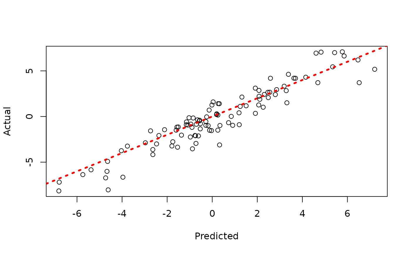

Now, suppose we want to analyze each of the chains separately to assess mixing / convergence.

We can use our knowledge of the internal arrangement of the chain samples to construct a an mcmc.list in the coda package, from which we can perform various diagnostics.

sigma2_coda_list <- coda::as.mcmc.list(lapply(
  1:num_chains,
  function(chain_idx) {
    offset <- (chain_idx - 1) * num_mcmc
    inds_start <- offset + 1
    inds_end <- offset + num_mcmc
    coda::mcmc(bart_model$sigma2_global_samples[inds_start:inds_end])
  }
))
traceplot(sigma2_coda_list, ylab = expression(sigma^2))
abline(h = noise_sd^2, col = "black", lty = 3, lwd = 3)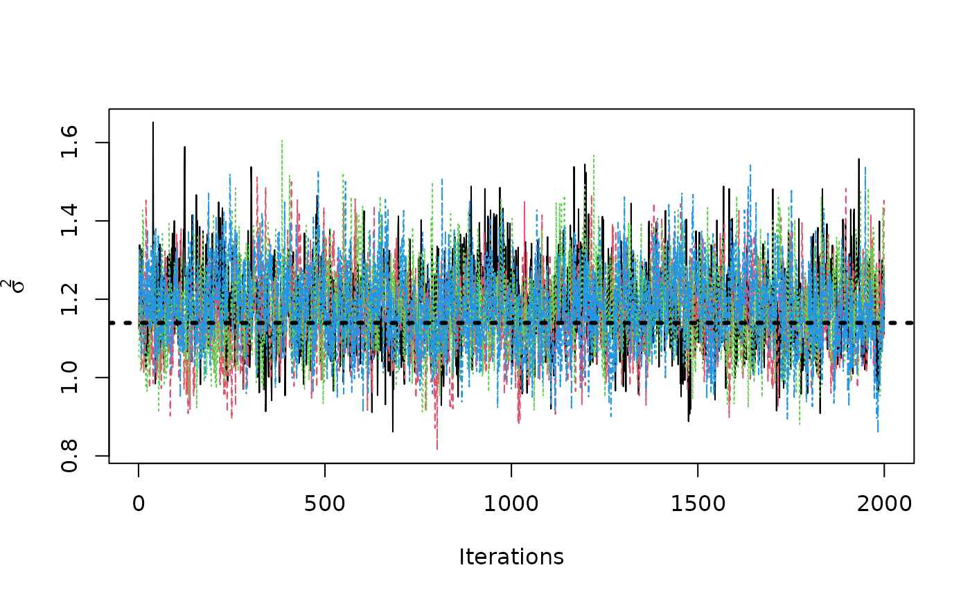

acf <- autocorr.diag(sigma2_coda_list)
ess <- effectiveSize(sigma2_coda_list)
rhat <- gelman.diag(sigma2_coda_list, autoburnin = F)
cat(paste0(
  "Average autocorrelation across chains:\n",
  paste0(paste0(rownames(acf), ": ", round(acf, 3)), collapse = ", "),
  "\nTotal effective sample size across chains: ",
  paste0(round(ess, 1), collapse = ", "),
  "\n'R-hat' potential scale reduction factor of Gelman and Rubin (1992)): ",
  paste0(
    round(rhat$psrf[, 1], 3),
    collapse = ", "
  )
))
#> Average autocorrelation across chains:
#> Lag 0: 1, Lag 1: 0.367, Lag 5: 0.117, Lag 10: 0.073, Lag 50: 0.034
#> Total effective sample size across chains: 1959
#> 'R-hat' potential scale reduction factor of Gelman and Rubin (1992)): 1.005

We can convert this to an array to be consumed by the bayesplot package

coda_array <- as.array(sigma2_coda_list)
dim(coda_array) <- c(nrow(coda_array), ncol(coda_array), 1)
dimnames(coda_array) <- list(
  Iteration = paste0("iter", 1:num_mcmc),
  Chain = paste0("chain", 1:num_chains),
  Parameter = "sigma2_global"
)

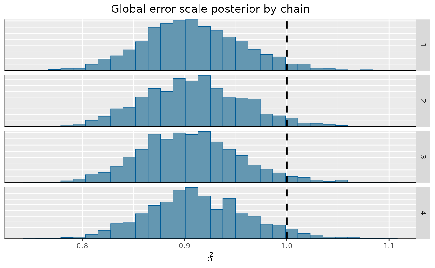
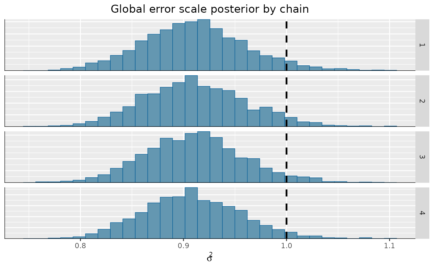
From here, we can visualize the posterior of $\sigma^2$ for each chain, comparing to the true simulated value.

bayesplot::mcmc_hist_by_chain(
  coda_array,
  pars = "sigma2_global"
) +
  ggplot2::labs(
    title = "Global error scale posterior by chain",
    x = expression(sigma^2)
  ) +
  ggplot2::theme(
    plot.title = ggplot2::element_text(hjust = 0.5)
  ) +
  ggplot2::geom_vline(
    xintercept = noise_sd^2,
    color = "black",
    linetype = "dashed",
    size = 1
  )

We can also analyze the pointwise forest predictions. Let’s consider 5 observations with the largest test-set residual.

abs_test_set_resid <- abs(y_test - y_hat_test)
top5_resids <- order(abs_test_set_resid, decreasing = T)[1:5]
y_hat_test_posterior <- predict(
  bart_model,
  X = X_test[top5_resids, ],
  leaf_basis = leaf_basis_test[top5_resids],
  type = "posterior",
  terms = "y_hat"
)
y_hat_coda_list <- coda::as.mcmc.list(lapply(1:num_chains, function(chain_idx) {
  offset <- (chain_idx - 1) * num_mcmc
  inds_start <- offset + 1
  inds_end <- offset + num_mcmc
  coda::mcmc(t(y_hat_test_posterior[, inds_start:inds_end]))
}))
acf <- autocorr.diag(y_hat_coda_list)
ess <- effectiveSize(y_hat_coda_list)
rhat <- gelman.diag(y_hat_coda_list)

cat(
  "Average autocorrelation across chains for each of five observations:\n",
  paste0(
    sapply(1:5, function(i) {
      paste0(
        "Observation ",
        top5_resids[i],
        ":\n",
        paste0(rownames(acf), ": ", round(acf[, i], 3), collapse = ", "),
        "\n"
      )
    })
  ),
  "\n",
  sep = ""
)
#> Average autocorrelation across chains for each of five observations:
#> Observation 41:
#> Lag 0: 1, Lag 1: 0.629, Lag 5: 0.394, Lag 10: 0.325, Lag 50: 0.224
#> Observation 82:
#> Lag 0: 1, Lag 1: 0.496, Lag 5: 0.196, Lag 10: 0.093, Lag 50: 0.028
#> Observation 32:
#> Lag 0: 1, Lag 1: 0.444, Lag 5: 0.205, Lag 10: 0.129, Lag 50: 0.033
#> Observation 63:
#> Lag 0: 1, Lag 1: 0.568, Lag 5: 0.213, Lag 10: 0.101, Lag 50: 0.042
#> Observation 93:
#> Lag 0: 1, Lag 1: 0.524, Lag 5: 0.254, Lag 10: 0.16, Lag 50: 0.035

cat(
  "Total effective sample size across chains:\n",
  paste0(
    sapply(1:5, function(i) {
      paste0(
        "Observation ",
        top5_resids[i],
        ": ",
        paste0(round(ess[i], 1), collapse = ", "),
        "\n"
      )
    })
  ),
  "\n",
  sep = ""
)
#> Total effective sample size across chains:
#> Observation 41: 393.4
#> Observation 82: 1446.4
#> Observation 32: 1236
#> Observation 63: 1243.9
#> Observation 93: 784.5

cat(
  "'R-hat' potential scale reduction factor of Gelman and Rubin (1992)\n",
  paste0(
    sapply(1:5, function(i) {
      paste0(
        "Observation ",
        top5_resids[i],
        ": ",
        paste0(round(rhat$psrf[i, 1], 3), collapse = ", "),
        "\n"
      )
    })
  ),
  sep = ""
)
#> 'R-hat' potential scale reduction factor of Gelman and Rubin (1992)
#> Observation 41: 1.156
#> Observation 82: 1.002
#> Observation 32: 1.005
#> Observation 63: 1.014
#> Observation 93: 1.003

We can see that these “hard to predict” observations have a higher autocorrelation and lower effective sample size.

Sampling Multiple Chains Sequentially from XBART forests

In the example above, each chain was initialized from “root”, meaning each tree in a forest was a single root node and all parameter values were set to a “default” starting point. If we sample a model using a small number of ‘grow-from-root’ iterations, we can use these forests to initialize MCMC chains.

num_chains <- 4
num_gfr <- 5
num_burnin <- 1000
num_mcmc <- 2000

Run the initial GFR sampler

xbart_model <- stochtree::bart(
  X_train = X_train,
  leaf_basis_train = leaf_basis_train,
  y_train = y_train,
  num_gfr = num_gfr,
  num_burnin = 0,
  num_mcmc = 0
)
xbart_model_string <- stochtree::saveBARTModelToJsonString(xbart_model)

Run the multi-chain BART sampler, with each chain initialized from a different GFR forest

bart_model <- stochtree::bart(
  X_train = X_train,
  leaf_basis_train = leaf_basis_train,
  y_train = y_train,
  num_gfr = num_gfr,
  num_burnin = num_burnin,
  num_mcmc = num_mcmc,
  general_params = list(num_chains = num_chains),
  previous_model_json = xbart_model_string,
  previous_model_warmstart_sample_num = num_gfr
)

Now we have a bartmodel object with num_chains * num_mcmc samples stored internally. These samples are arranged sequentially, with the first num_mcmc samples corresponding to chain 1, the next num_mcmc samples to chain 2, etc…

Since each chain is a set of samples of the same model, we can analyze the samples collectively, for example, by looking at out-of-sample predictions.

y_hat_test <- predict(
  bart_model,
  X = X_test,
  leaf_basis = leaf_basis_test,
  type = "mean",
  terms = "y_hat"
)
plot(y_hat_test, y_test, xlab = "Predicted", ylab = "Actual")
abline(0, 1, col = "red", lty = 3, lwd = 3)

Now, suppose we want to analyze each of the chains separately to assess mixing / convergence.

We can use our knowledge of the internal arrangement of the chain samples to construct a an mcmc.list in the coda package, from which we can perform various diagnostics.

sigma2_coda_list <- coda::as.mcmc.list(lapply(
  1:num_chains,
  function(chain_idx) {
    offset <- (chain_idx - 1) * num_mcmc
    inds_start <- offset + 1
    inds_end <- offset + num_mcmc
    coda::mcmc(bart_model$sigma2_global_samples[inds_start:inds_end])
  }
))
traceplot(sigma2_coda_list, ylab = expression(sigma^2))
abline(h = noise_sd^2, col = "black", lty = 3, lwd = 3)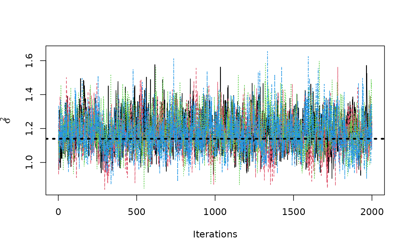

acf <- autocorr.diag(sigma2_coda_list)
ess <- effectiveSize(sigma2_coda_list)
rhat <- gelman.diag(sigma2_coda_list, autoburnin = F)
cat(paste0(
  "Average autocorrelation across chains:\n",
  paste0(paste0(rownames(acf), ": ", round(acf, 3)), collapse = ", "),
  "\nTotal effective sample size across chains: ",
  paste0(round(ess, 1), collapse = ", "),
  "\n'R-hat' potential scale reduction factor of Gelman and Rubin (1992)): ",
  paste0(
    round(rhat$psrf[, 1], 3),
    collapse = ", "
  )
))
#> Average autocorrelation across chains:
#> Lag 0: 1, Lag 1: 0.359, Lag 5: 0.132, Lag 10: 0.089, Lag 50: 0.027
#> Total effective sample size across chains: 1730.3
#> 'R-hat' potential scale reduction factor of Gelman and Rubin (1992)): 1.008

We can convert this to an array to be consumed by the bayesplot package

coda_array <- as.array(sigma2_coda_list)
dim(coda_array) <- c(nrow(coda_array), ncol(coda_array), 1)
dimnames(coda_array) <- list(
  Iteration = paste0("iter", 1:num_mcmc),
  Chain = paste0("chain", 1:num_chains),
  Parameter = "sigma2_global"
)

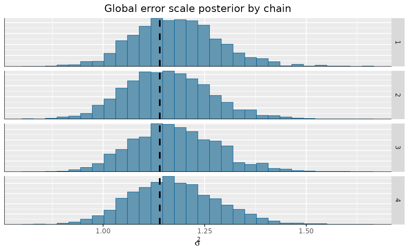
From here, we can visualize the posterior of $\sigma^2$ for each chain, comparing to the true simulated value.

bayesplot::mcmc_hist_by_chain(
  coda_array,
  pars = "sigma2_global"
) +
  ggplot2::labs(
    title = "Global error scale posterior by chain",
    x = expression(sigma^2)
  ) +
  ggplot2::theme(
    plot.title = ggplot2::element_text(hjust = 0.5)
  ) +
  ggplot2::geom_vline(
    xintercept = noise_sd^2,
    color = "black",
    linetype = "dashed",
    size = 1
  )

We can also analyze the pointwise forest predictions. Let’s consider 5 observations with the largest test-set residual.

abs_test_set_resid <- abs(y_test - y_hat_test)
top5_resids <- order(abs_test_set_resid, decreasing = T)[1:5]
y_hat_test_posterior <- predict(
  bart_model,
  X = X_test[top5_resids, ],
  leaf_basis = leaf_basis_test[top5_resids],
  type = "posterior",
  terms = "y_hat"
)
y_hat_coda_list <- coda::as.mcmc.list(lapply(1:num_chains, function(chain_idx) {
  offset <- (chain_idx - 1) * num_mcmc
  inds_start <- offset + 1
  inds_end <- offset + num_mcmc
  coda::mcmc(t(y_hat_test_posterior[, inds_start:inds_end]))
}))
acf <- autocorr.diag(y_hat_coda_list)
ess <- effectiveSize(y_hat_coda_list)
rhat <- gelman.diag(y_hat_coda_list)

cat(
  "Average autocorrelation across chains for each of five observations:\n",
  paste0(
    sapply(1:5, function(i) {
      paste0(
        "Observation ",
        top5_resids[i],
        ":\n",
        paste0(rownames(acf), ": ", round(acf[, i], 3), collapse = ", "),
        "\n"
      )
    })
  ),
  "\n",
  sep = ""
)
#> Average autocorrelation across chains for each of five observations:
#> Observation 41:
#> Lag 0: 1, Lag 1: 0.635, Lag 5: 0.403, Lag 10: 0.344, Lag 50: 0.259
#> Observation 82:
#> Lag 0: 1, Lag 1: 0.492, Lag 5: 0.194, Lag 10: 0.112, Lag 50: 0.018
#> Observation 32:
#> Lag 0: 1, Lag 1: 0.45, Lag 5: 0.195, Lag 10: 0.117, Lag 50: 0.03
#> Observation 93:
#> Lag 0: 1, Lag 1: 0.516, Lag 5: 0.24, Lag 10: 0.142, Lag 50: 0.042
#> Observation 63:
#> Lag 0: 1, Lag 1: 0.572, Lag 5: 0.243, Lag 10: 0.152, Lag 50: 0.014

cat(
  "Total effective sample size across chains:\n",
  paste0(
    sapply(1:5, function(i) {
      paste0(
        "Observation ",
        top5_resids[i],
        ": ",
        paste0(round(ess[i], 1), collapse = ", "),
        "\n"
      )
    })
  ),
  "\n",
  sep = ""
)
#> Total effective sample size across chains:
#> Observation 41: 338.3
#> Observation 82: 1334.9
#> Observation 32: 1220.3
#> Observation 93: 1075.5
#> Observation 63: 1025.4

cat(
  "'R-hat' potential scale reduction factor of Gelman and Rubin (1992)\n",
  paste0(
    sapply(1:5, function(i) {
      paste0(
        "Observation ",
        top5_resids[i],
        ": ",
        paste0(round(rhat$psrf[i, 1], 3), collapse = ", "),
        "\n"
      )
    })
  ),
  sep = ""
)
#> 'R-hat' potential scale reduction factor of Gelman and Rubin (1992)
#> Observation 41: 1.032
#> Observation 82: 1.003
#> Observation 32: 1.006
#> Observation 93: 1.017
#> Observation 63: 1.01

We can see that some of these “hard to predict” observations have a higher autocorrelation and lower effective sample size.

Sampling Multiple Chains in Parallel

The above example was made somewhat straightforward by the fact that bart() and bcf() both allow for sequential multi-chain sampling internally. While we do not currently support parallel multi-chain sampling internally in the bart() and bcf() functions, it is possible to do this via doParallel. While bartmodel or bcfmodel objects contain external pointers to C++ data structures (i.e. decision tree ensembles) which are not reachable by other processes, we can serialize stochtree models to JSON for cross-process communication. After num_chains models have been run in parallel and their JSON representations have been collated in the primary R session, we can combine these into a single bartmodel or bcfmodel object via the createBARTModelFromCombinedJsonString() or createBCFModelFromCombinedJsonString() functions.

In order to run multiple parallel stochtree chains, a parallel backend must be registered in your R environment. The code below will register a parallel backend with access to as many cores are available on your machine. Note that we do not evaluate the code snippet below in order to interact nicely with CRAN / Github Actions environments.

ncores <- parallel::detectCores()
cl <- makeCluster(ncores)
registerDoParallel(cl)

Note that the bartmodel object contains external pointers to forests created by the stochtree shared object, and when stochtree::bart() is run in parallel on independent subprocesses, these pointers are not generally accessible in the session that kicked off the parallel run.

To overcome this, you can return a JSON representation of a bartmodel in memory and combine them into a single in-memory bartmodel object.

The first step of this process is to run the sampler in parallel, storing the resulting BART JSON strings in a list.

num_chains <- 4
num_gfr <- 0
num_burnin <- 100
num_mcmc <- 100

bart_model_outputs <- foreach(i = 1:num_chains) %dopar%
  {
    random_seed <- i
    general_params <- list(sample_sigma2_global = T, random_seed = random_seed)
    mean_forest_params <- list(sample_sigma2_leaf = F)
    bart_model <- stochtree::bart(
      X_train = X_train,
      leaf_basis_train = leaf_basis_train,
      y_train = y_train,
      X_test = X_test,
      leaf_basis_test = leaf_basis_test,
      num_gfr = num_gfr,
      num_burnin = num_burnin,
      num_mcmc = num_mcmc,
      general_params = general_params,
      mean_forest_params = mean_forest_params
    )
    bart_model_string <- stochtree::saveBARTModelToJsonString(bart_model)
    y_hat_test <- bart_model$y_hat_test
    list(model = bart_model_string, yhat = y_hat_test)
  }
#> Warning: executing %dopar% sequentially: no parallel backend registered

Close the parallel cluster (not evaluated here, as explained above).

stopCluster(cl)

Now, if we want to combine the forests from each of these BART models into a single forest, we can do so as follows

bart_model_strings <- list()
bart_model_yhats <- matrix(NA, nrow = length(y_test), ncol = num_chains)
for (i in 1:length(bart_model_outputs)) {
  bart_model_strings[[i]] <- bart_model_outputs[[i]]$model
  bart_model_yhats[, i] <- rowMeans(bart_model_outputs[[i]]$yhat)
}
combined_bart <- createBARTModelFromCombinedJsonString(bart_model_strings)

We can predict from this combined forest as follows

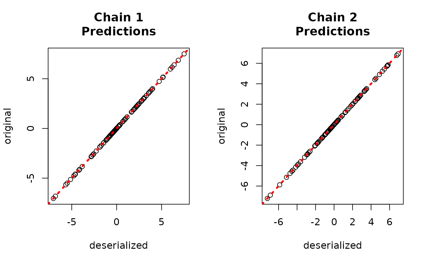
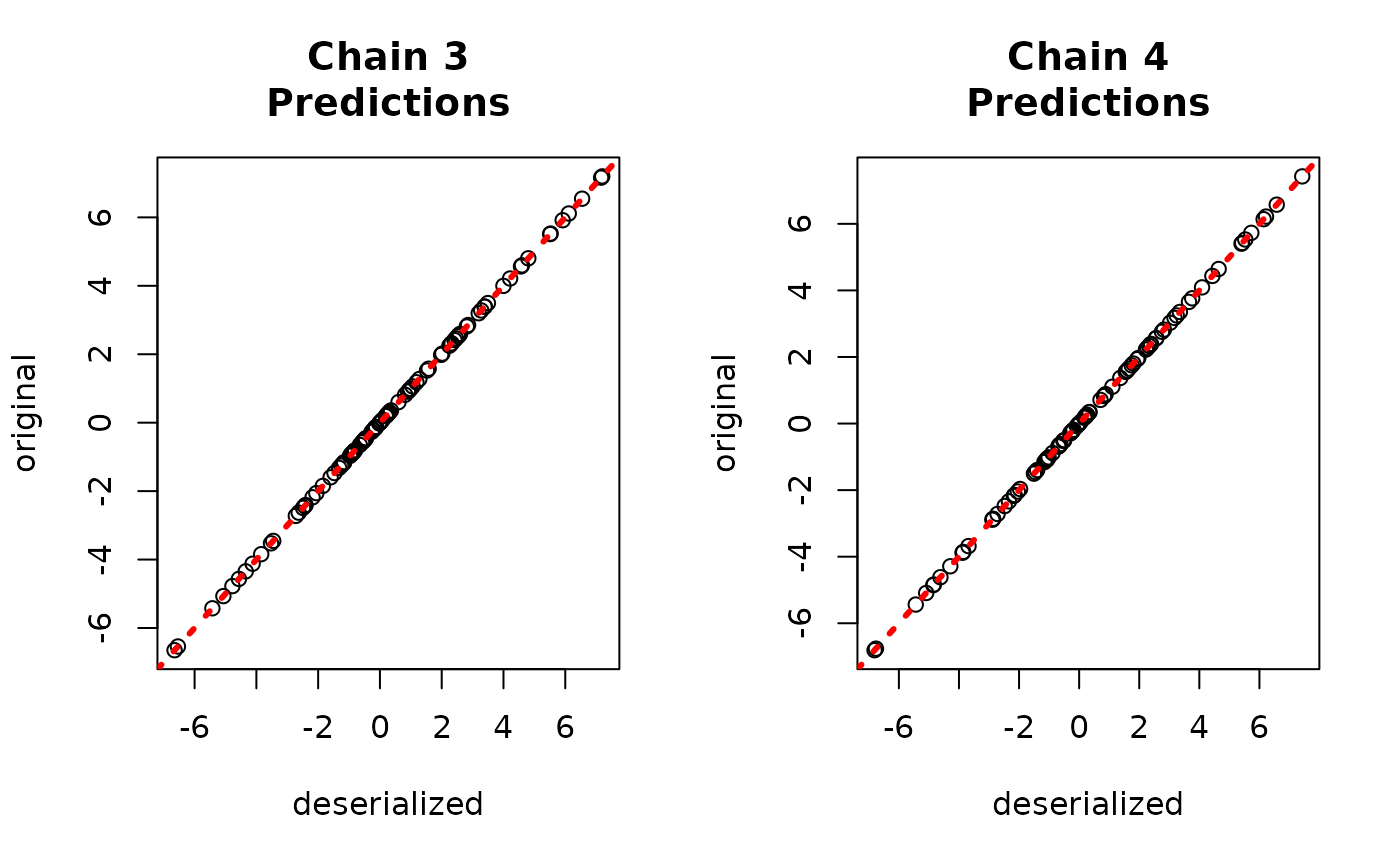
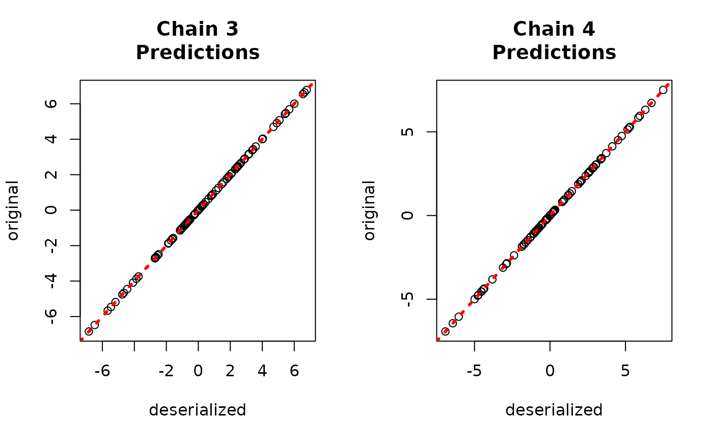
yhat_combined <- predict(combined_bart, X_test, leaf_basis_test)$y_hat

Compare average predictions from each chain to the original predictions.

par(mfrow = c(1, 2))
for (i in 1:num_chains) {
  offset <- (i - 1) * num_mcmc
  inds_start <- offset + 1
  inds_end <- offset + num_mcmc
  plot(
    rowMeans(yhat_combined[, inds_start:inds_end]),
    bart_model_yhats[, i],
    xlab = "deserialized",
    ylab = "original",
    main = paste0("Chain ", i, "\nPredictions")
  )
  abline(0, 1, col = "red", lty = 3, lwd = 3)
}

par(mfrow = c(1, 1))

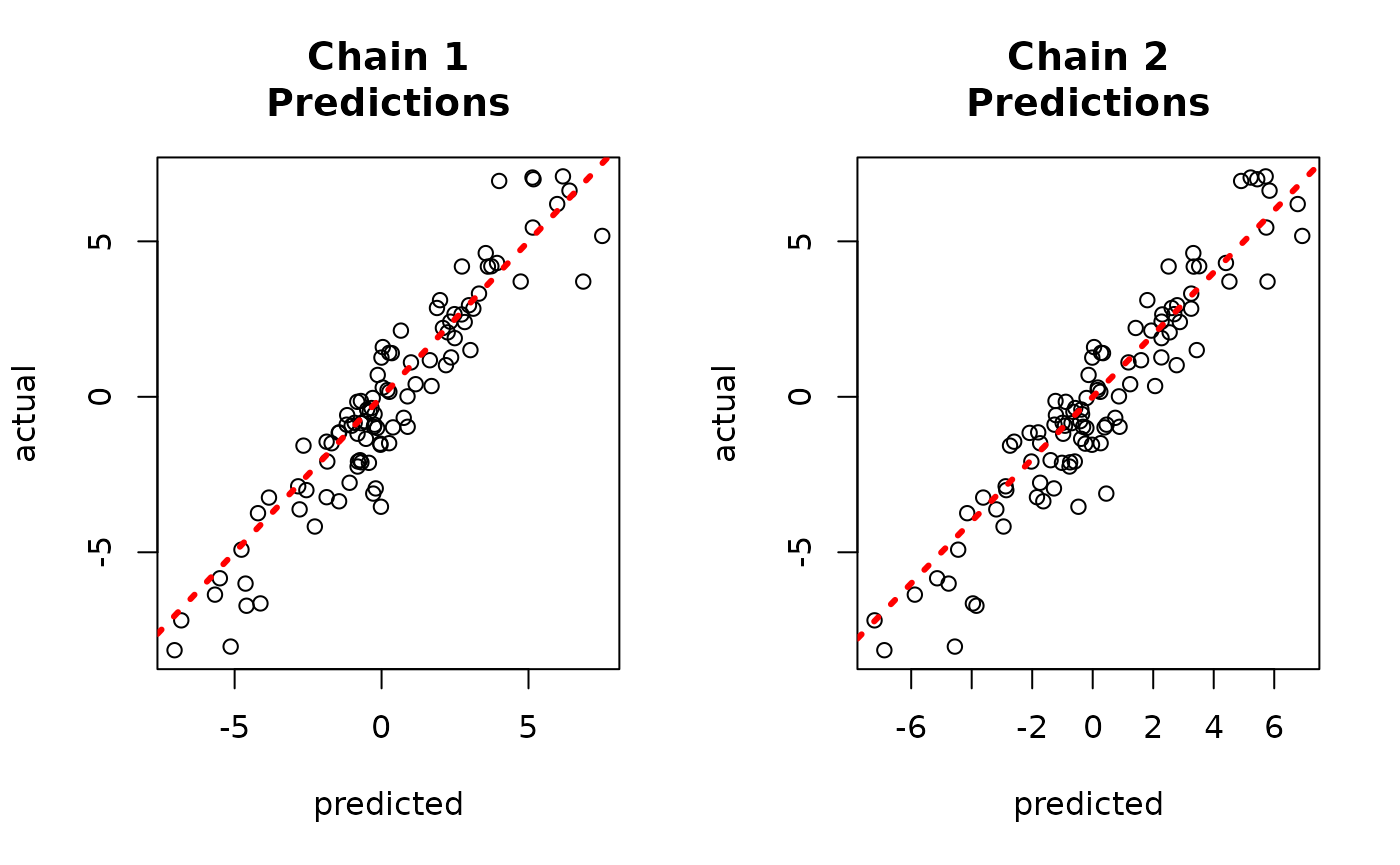
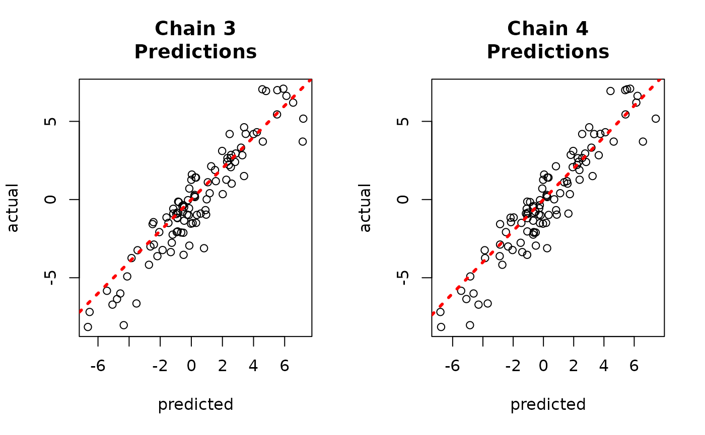
And to the true $y$ values.

par(mfrow = c(1, 2))
for (i in 1:num_chains) {
  offset <- (i - 1) * num_mcmc
  inds_start <- offset + 1
  inds_end <- offset + num_mcmc
  plot(
    rowMeans(yhat_combined[, inds_start:inds_end]),
    y_test,
    xlab = "predicted",
    ylab = "actual",
    main = paste0("Chain ", i, "\nPredictions")
  )
  abline(0, 1, col = "red", lty = 3, lwd = 3)
}

par(mfrow = c(1, 1))

Warmstarting Multiple Chains in Parallel

In the above example, we ran multiple parallel chains with each MCMC sampler starting from a “root” forest. Consider instead the “warmstart” approach of He and Hahn (2023), where forests are sampled using the fast “grow-from-root” (GFR) algorithm and then several MCMC chains are run using different GFR forests.

First, we sample this model using the grow-from-root algorithm in the main R session for several iterations (we will use these forests to see independent parallel chains in a moment).

num_chains <- 4
num_gfr <- 5
num_burnin <- 100
num_mcmc <- 100

general_params <- list(sample_sigma2_global = T)
mean_forest_params <- list(sample_sigma2_leaf = T)
xbart_model <- stochtree::bart(
  X_train = X_train,
  leaf_basis_train = leaf_basis_train,
  y_train = y_train,
  X_test = X_test,
  leaf_basis_test = leaf_basis_test,
  num_gfr = num_gfr,
  num_burnin = 0,
  num_mcmc = 0,
  general_params = general_params,
  mean_forest_params = mean_forest_params
)
xbart_model_string <- stochtree::saveBARTModelToJsonString(xbart_model)

In order to run this sampler in parallel, a parallel backend must be registered in your R environment. The code below will register a parallel backend with access to as many cores are available on your machine. Note that we do not evaluate the code snippet below in order to interact nicely with CRAN / Github Actions environments.

ncores <- parallel::detectCores()
cl <- makeCluster(ncores)
registerDoParallel(cl)

Note that the bartmodel object contains external pointers to forests created by the stochtree shared object, and when stochtree::bart() is run in parallel on independent subprocesses, these pointers are not generally accessible in the session that kicked off the parallel run.

To overcome this, you can return a JSON representation of a bartmodel in memory and combine them into a single in-memory bartmodel object.

The first step of this process is to run the sampler in parallel, storing the resulting BART JSON strings in a list.

bart_model_outputs <- foreach(i = 1:num_chains) %dopar%
  {
    random_seed <- i
    general_params <- list(sample_sigma2_global = T, random_seed = random_seed)
    mean_forest_params <- list(sample_sigma2_leaf = T)
    bart_model <- stochtree::bart(
      X_train = X_train,
      leaf_basis_train = leaf_basis_train,
      y_train = y_train,
      X_test = X_test,
      leaf_basis_test = leaf_basis_test,
      num_gfr = 0,
      num_burnin = num_burnin,
      num_mcmc = num_mcmc,
      general_params = general_params,
      mean_forest_params = mean_forest_params,
      previous_model_json = xbart_model_string,
      previous_model_warmstart_sample_num = num_gfr - i + 1,
    )
    bart_model_string <- stochtree::saveBARTModelToJsonString(bart_model)
    y_hat_test <- bart_model$y_hat_test
    list(model = bart_model_string, yhat = y_hat_test)
  }

Close the parallel cluster (not evaluated here, as explained above).

stopCluster(cl)

Now, if we want to combine the forests from each of these BART models into a single forest, we can do so as follows

bart_model_strings <- list()
bart_model_yhats <- matrix(NA, nrow = length(y_test), ncol = num_chains)
for (i in 1:length(bart_model_outputs)) {
  bart_model_strings[[i]] <- bart_model_outputs[[i]]$model
  bart_model_yhats[, i] <- rowMeans(bart_model_outputs[[i]]$yhat)
}
combined_bart <- createBARTModelFromCombinedJsonString(bart_model_strings)

We can predict from this combined forest as follows

yhat_combined <- predict(combined_bart, X_test, leaf_basis_test)$y_hat

Compare average predictions from each chain to the original predictions.

par(mfrow = c(1, 2))
for (i in 1:num_chains) {
  offset <- (i - 1) * num_mcmc
  inds_start <- offset + 1
  inds_end <- offset + num_mcmc
  plot(
    rowMeans(yhat_combined[, inds_start:inds_end]),
    bart_model_yhats[, i],
    xlab = "deserialized",
    ylab = "original",
    main = paste0("Chain ", i, "\nPredictions")
  )
  abline(0, 1, col = "red", lty = 3, lwd = 3)
}

par(mfrow = c(1, 1))

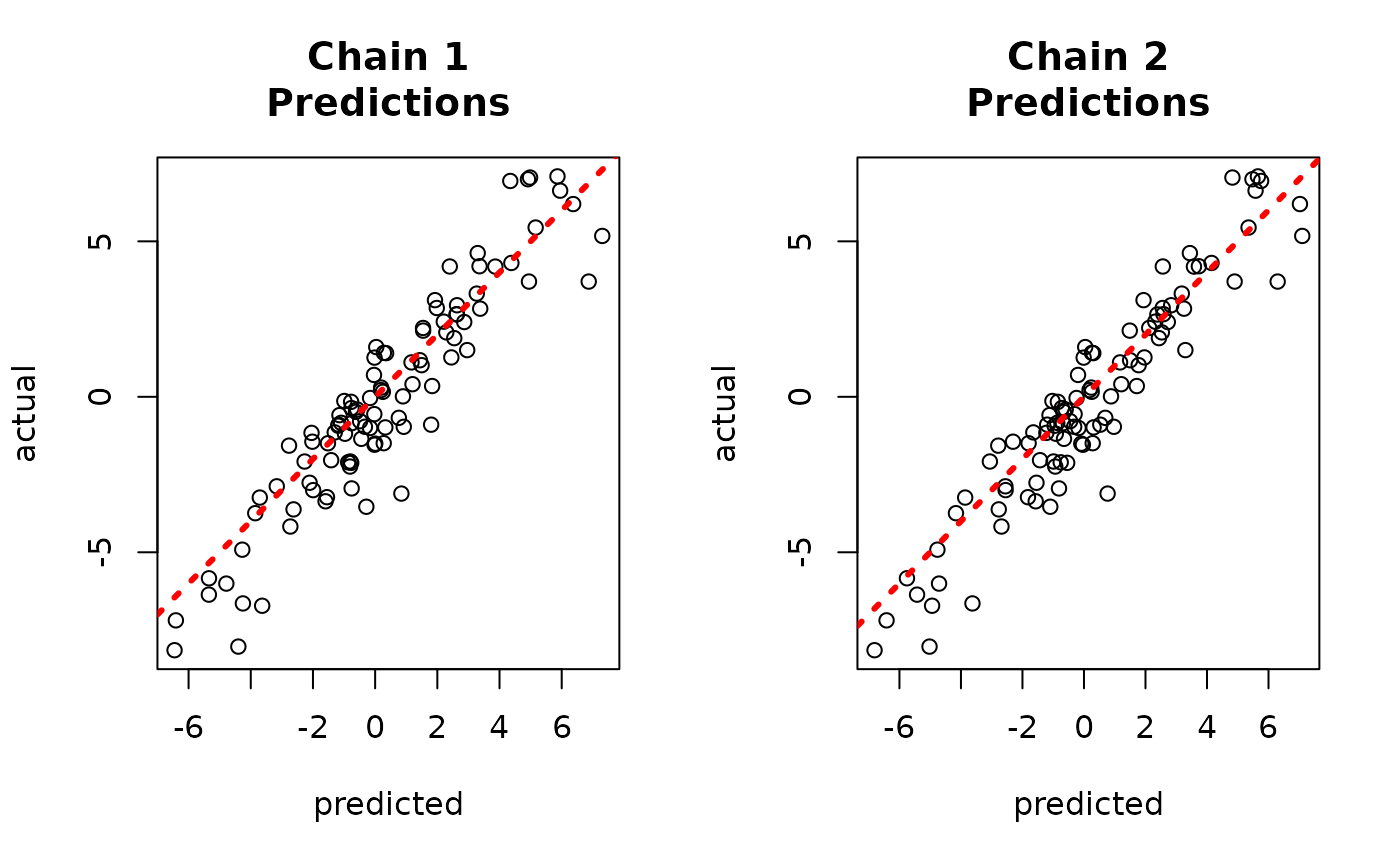
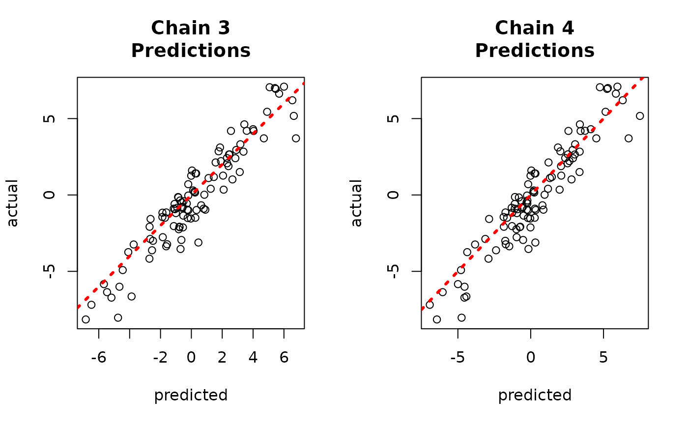
And to the true $y$ values.

par(mfrow = c(1, 2))
for (i in 1:num_chains) {
  offset <- (i - 1) * num_mcmc
  inds_start <- offset + 1
  inds_end <- offset + num_mcmc
  plot(
    rowMeans(yhat_combined[, inds_start:inds_end]),
    y_test,
    xlab = "predicted",
    ylab = "actual",
    main = paste0("Chain ", i, "\nPredictions")
  )
  abline(0, 1, col = "red", lty = 3, lwd = 3)
}

par(mfrow = c(1, 1))

Demo 2: Causal Inference

Data Simulation

Simulate a simple causal model

# Generate the data
n <- 1000
p <- 5
X <- matrix(runif(n * p), ncol = p)
pi_x <- 0.25 + 0.5 * X[, 1]
mu_x <- pi_x * 5 + 2 * X[, 3]
tau_x <- X[, 2] * 2 - 1
Z <- rbinom(n, 1, pi_x)
E_Y_XZ <- mu_x + tau_x * Z
y <- E_Y_XZ + rnorm(n, 0, 1)

# Split data into test and train sets
test_set_pct <- 0.2
n_test <- round(test_set_pct * n)
n_train <- n - n_test
test_inds <- sort(sample(1:n, n_test, replace = FALSE))
train_inds <- (1:n)[!((1:n) %in% test_inds)]
X_test <- X[test_inds, ]
X_train <- X[train_inds, ]
Z_test <- Z[test_inds]
Z_train <- Z[train_inds]
propensity_test <- pi_x[test_inds]
propensity_train <- pi_x[train_inds]
y_test <- y[test_inds]
y_train <- y[train_inds]

Sampling Multiple Chains Sequentially from Scratch

As with the supervised learning (BART) demo, we run 4 independent chains with 2000 MCMC iterations, each of which is burned in for 1000 iterations.

num_chains <- 4
num_gfr <- 0
num_burnin <- 1000
num_mcmc <- 2000

Run the sampler

general_params <- list(
  num_chains = num_chains
)
bcf_model <- stochtree::bcf(
  X_train = X_train,
  Z_train = Z_train,
  propensity_train = propensity_train,
  y_train = y_train,
  num_gfr = num_gfr,
  num_burnin = num_burnin,
  num_mcmc = num_mcmc,
  general_params = general_params
)

Now we have a bcfmodel object with num_chains * num_mcmc samples stored internally. These samples are arranged sequentially, with the first num_mcmc samples corresponding to chain 1, the next num_mcmc samples to chain 2, etc…

Since each chain is a set of samples of the same model, we can analyze the samples collectively, for example, by looking at out-of-sample predictions.

y_hat_test <- predict(
  bcf_model,
  X = X_test,
  Z = Z_test,
  propensity = propensity_test,
  type = "mean",
  terms = "y_hat"
)
plot(y_hat_test, y_test, xlab = "Predicted", ylab = "Actual")
abline(0, 1, col = "red", lty = 3, lwd = 3)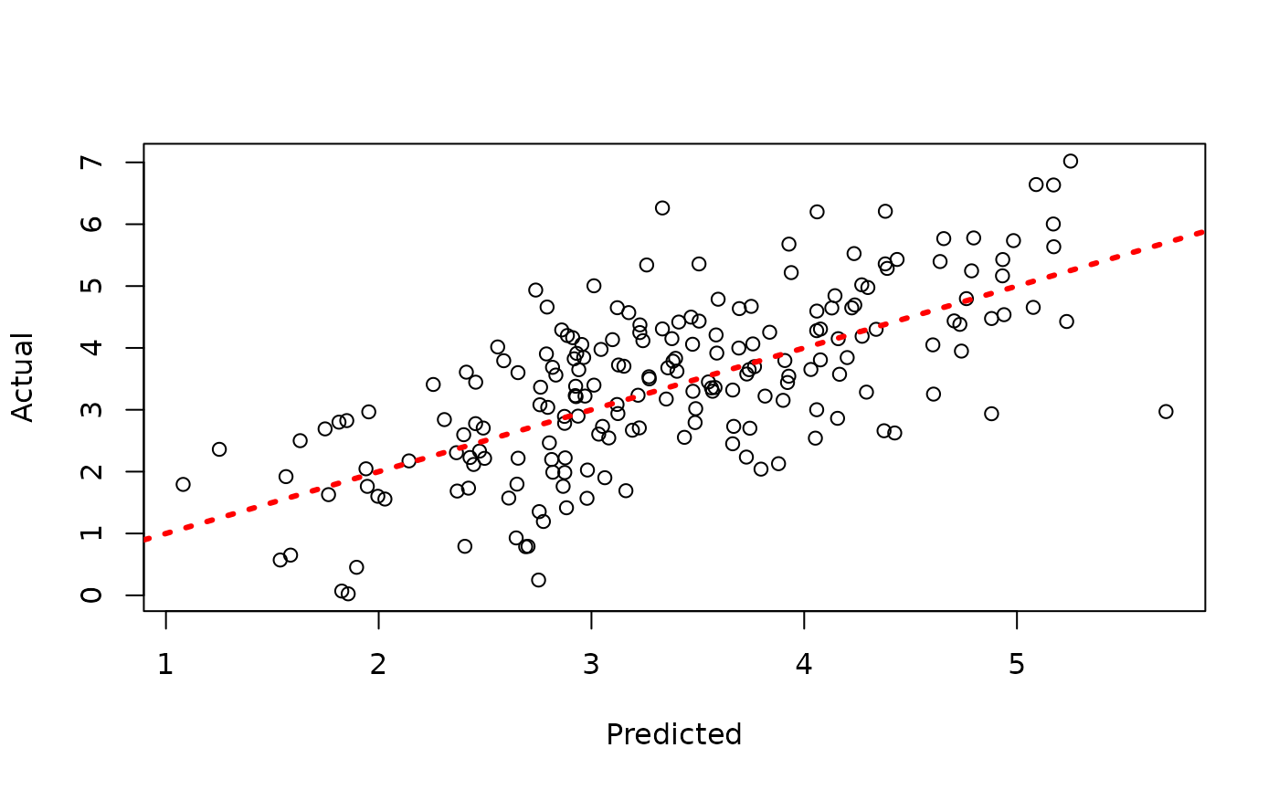

Now, suppose we want to analyze each of the chains separately to assess mixing / convergence.

We can use our knowledge of the internal arrangement of the chain samples to construct a an mcmc.list in the coda package, from which we can perform various diagnostics.

sigma2_coda_list <- coda::as.mcmc.list(lapply(
  1:num_chains,
  function(chain_idx) {
    offset <- (chain_idx - 1) * num_mcmc
    inds_start <- offset + 1
    inds_end <- offset + num_mcmc
    coda::mcmc(bcf_model$sigma2_global_samples[inds_start:inds_end])
  }
))
traceplot(sigma2_coda_list, ylab = expression(sigma^2))
abline(h = 1, col = "black", lty = 3, lwd = 3)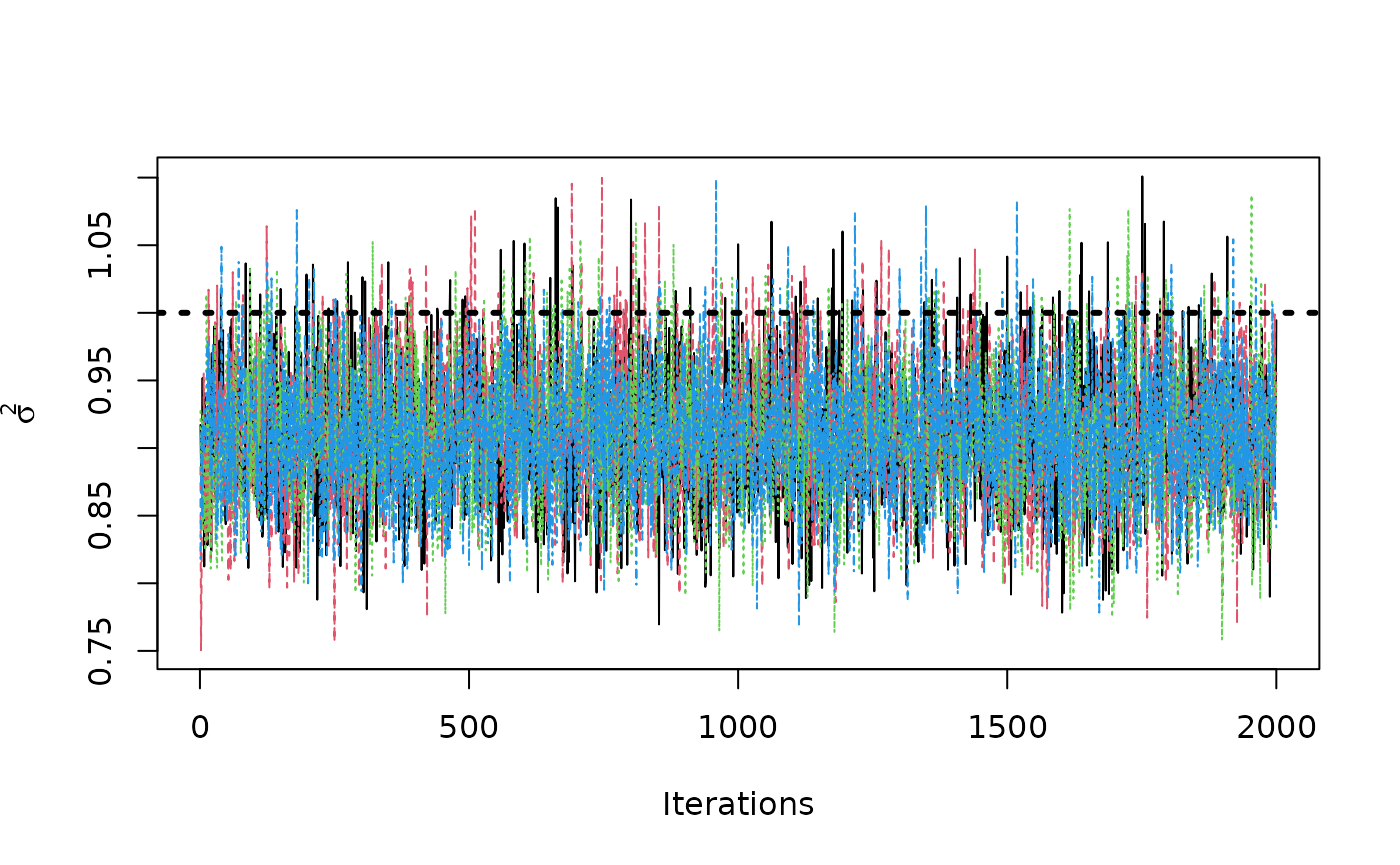

acf <- autocorr.diag(sigma2_coda_list)
ess <- effectiveSize(sigma2_coda_list)
rhat <- gelman.diag(sigma2_coda_list, autoburnin = F)
cat(paste0(
  "Average autocorrelation across chains:\n",
  paste0(paste0(rownames(acf), ": ", round(acf, 3)), collapse = ", "),
  "\nTotal effective sample size across chains: ",
  paste0(round(ess, 1), collapse = ", "),
  "\n'R-hat' potential scale reduction factor of Gelman and Rubin (1992)): ",
  paste0(
    round(rhat$psrf[, 1], 3),
    collapse = ", "
  )
))
#> Average autocorrelation across chains:
#> Lag 0: 1, Lag 1: 0.118, Lag 5: 0.011, Lag 10: 0.007, Lag 50: -0.01
#> Total effective sample size across chains: 5600.8
#> 'R-hat' potential scale reduction factor of Gelman and Rubin (1992)): 1.001

We can convert this to an array to be consumed by the bayesplot package

coda_array <- as.array(sigma2_coda_list)
dim(coda_array) <- c(nrow(coda_array), ncol(coda_array), 1)
dimnames(coda_array) <- list(
  Iteration = paste0("iter", 1:num_mcmc),
  Chain = paste0("chain", 1:num_chains),
  Parameter = "sigma2_global"
)

From here, we can visualize the posterior of $\sigma^2$ for each chain, comparing to the true simulated value.

bayesplot::mcmc_hist_by_chain(
  coda_array,
  pars = "sigma2_global"
) +
  ggplot2::labs(
    title = "Global error scale posterior by chain",
    x = expression(sigma^2)
  ) +
  ggplot2::theme(
    plot.title = ggplot2::element_text(hjust = 0.5)
  ) +
  ggplot2::geom_vline(
    xintercept = 1,
    color = "black",
    linetype = "dashed",
    size = 1
  )

Sampling Multiple Chains Sequentially from XBCF Forests

As with the second supervised learning (BART) demo, we run 4 independent chains with 2000 MCMC iterations, each of which is burned in for 1000 iterations after being initialized from a different GFR forest.

num_chains <- 4
num_gfr <- 5
num_burnin <- 1000
num_mcmc <- 2000

Run the initial GFR sampler

xbcf_model <- stochtree::bcf(
  X_train = X_train,
  Z_train = Z_train,
  propensity_train = propensity_train,
  y_train = y_train,
  num_gfr = num_gfr,
  num_burnin = 0,
  num_mcmc = 0
)
xbcf_model_string <- stochtree::saveBCFModelToJsonString(xbcf_model)

Run the multi-chain BCF sampler, with each chain initialized from a different GFR forest

general_params <- list(
  num_chains = num_chains
)
bcf_model <- stochtree::bcf(
  X_train = X_train,
  Z_train = Z_train,
  propensity_train = propensity_train,
  y_train = y_train,
  num_gfr = 0,
  num_burnin = num_burnin,
  num_mcmc = num_mcmc,
  general_params = general_params,
  previous_model_json = xbcf_model_string,
  previous_model_warmstart_sample_num = num_gfr
)

Now we have a bcfmodel object with num_chains * num_mcmc samples stored internally. These samples are arranged sequentially, with the first num_mcmc samples corresponding to chain 1, the next num_mcmc samples to chain 2, etc…

Since each chain is a set of samples of the same model, we can analyze the samples collectively, for example, by looking at out-of-sample predictions.

y_hat_test <- predict(
  bcf_model,
  X = X_test,
  Z = Z_test,
  propensity = propensity_test,
  type = "mean",
  terms = "y_hat"
)
plot(y_hat_test, y_test, xlab = "Predicted", ylab = "Actual")
abline(0, 1, col = "red", lty = 3, lwd = 3)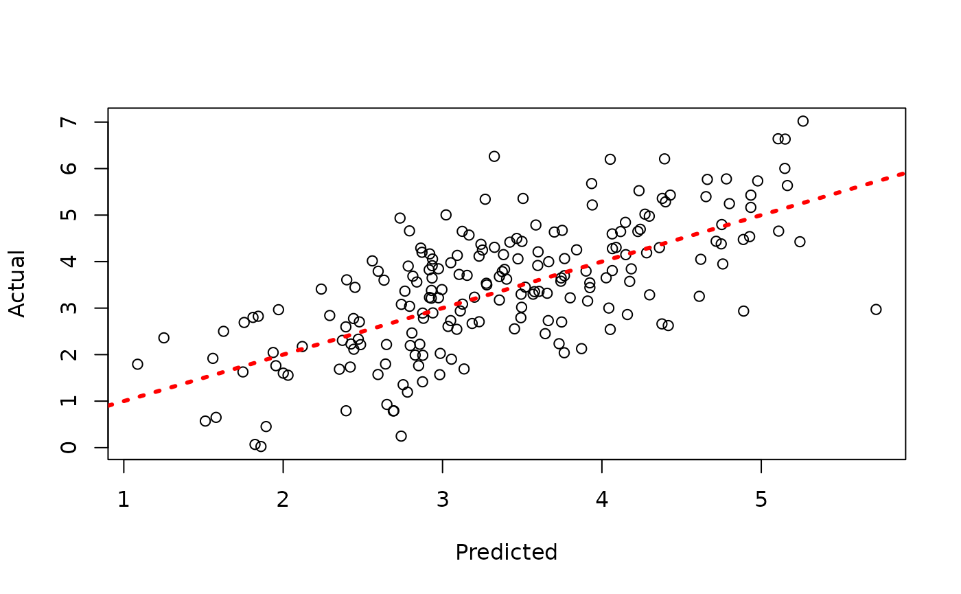

Now, suppose we want to analyze each of the chains separately to assess mixing / convergence.

We can use our knowledge of the internal arrangement of the chain samples to construct a an mcmc.list in the coda package, from which we can perform various diagnostics.

sigma2_coda_list <- coda::as.mcmc.list(lapply(
  1:num_chains,
  function(chain_idx) {
    offset <- (chain_idx - 1) * num_mcmc
    inds_start <- offset + 1
    inds_end <- offset + num_mcmc
    coda::mcmc(bcf_model$sigma2_global_samples[inds_start:inds_end])
  }
))
traceplot(sigma2_coda_list, ylab = expression(sigma^2))
abline(h = 1, col = "black", lty = 3, lwd = 3)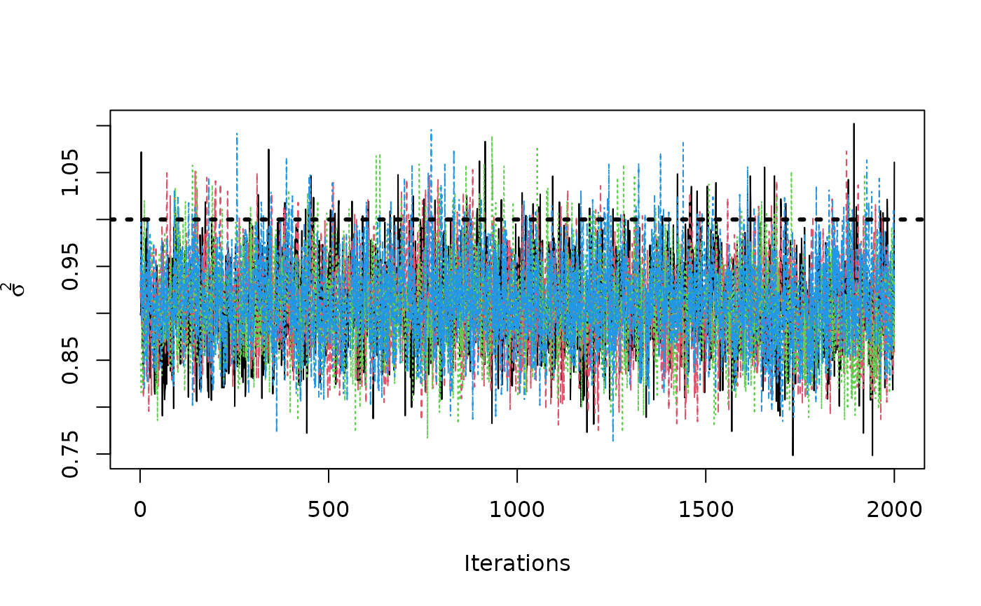

acf <- autocorr.diag(sigma2_coda_list)
ess <- effectiveSize(sigma2_coda_list)
rhat <- gelman.diag(sigma2_coda_list, autoburnin = F)
cat(paste0(
  "Average autocorrelation across chains:\n",
  paste0(paste0(rownames(acf), ": ", round(acf, 3)), collapse = ", "),
  "\nTotal effective sample size across chains: ",
  paste0(round(ess, 1), collapse = ", "),
  "\n'R-hat' potential scale reduction factor of Gelman and Rubin (1992)): ",
  paste0(
    round(rhat$psrf[, 1], 3),
    collapse = ", "
  )
))
#> Average autocorrelation across chains:
#> Lag 0: 1, Lag 1: 0.119, Lag 5: 0.034, Lag 10: 0.017, Lag 50: 0.01
#> Total effective sample size across chains: 4590.1
#> 'R-hat' potential scale reduction factor of Gelman and Rubin (1992)): 1.002

We can convert this to an array to be consumed by the bayesplot package

coda_array <- as.array(sigma2_coda_list)
dim(coda_array) <- c(nrow(coda_array), ncol(coda_array), 1)
dimnames(coda_array) <- list(
  Iteration = paste0("iter", 1:num_mcmc),
  Chain = paste0("chain", 1:num_chains),
  Parameter = "sigma2_global"
)

From here, we can visualize the posterior of $\sigma^2$ for each chain, comparing to the true simulated value.

bayesplot::mcmc_hist_by_chain(
  coda_array,
  pars = "sigma2_global"
) +
  ggplot2::labs(
    title = "Global error scale posterior by chain",
    x = expression(sigma^2)
  ) +
  ggplot2::theme(
    plot.title = ggplot2::element_text(hjust = 0.5)
  ) +
  ggplot2::geom_vline(
    xintercept = 1,
    color = "black",
    linetype = "dashed",
    size = 1
  )

References

Chipman, Hugh A., Edward I. George, and Robert E. McCulloch. 2010. “BART: Bayesian additive regression trees.” The Annals of Applied Statistics 4 (1): 266–98. https://doi.org/10.1214/09-AOAS285.

He, Jingyu, and P Richard Hahn. 2023. “Stochastic Tree Ensembles for Regularized Nonlinear Regression.” Journal of the American Statistical Association 118 (541): 551–70.

Krantsevich, Nikolay, Jingyu He, and P Richard Hahn. 2023. “Stochastic Tree Ensembles for Estimating Heterogeneous Effects.” In International Conference on Artificial Intelligence and Statistics, 6120–31. PMLR.