Bayesian Supervised Learning with Heteroskedasticity in StochTree

This vignette demonstrates how to use the bart() function for Bayesian supervised learning (Chipman, George, and McCulloch (2010)) and causal inference (Hahn, Murray, and Carvalho (2020)), with an additional “variance forest,” for modeling conditional variance (see Murray (2021)). To begin, we load the stochtree package.

library(stochtree)

Section 1: Supervised Learning

Demo 1: Variance-Only Simulation (simple DGP)

Simulation

Here, we generate data with a constant (zero) mean and a relatively simple covariate-modified variance function.

$$\begin{equation*} \begin{aligned} y &= 0 + \sigma(X) \epsilon\\ \sigma^2(X) &= \begin{cases} 0.5 & X_1 \geq 0 \text{ and } X_1 < 0.25\\ 1 & X_1 \geq 0.25 \text{ and } X_1 < 0.5\\ 2 & X_1 \geq 0.5 \text{ and } X_1 < 0.75\\ 3 & X_1 \geq 0.75 \text{ and } X_1 < 1\\ \end{cases}\\ X_1,\dots,X_p &\sim \text{U}\left(0,1\right)\\ \epsilon &\sim \mathcal{N}\left(0,1\right) \end{aligned} \end{equation*}$$

# Generate the data
n <- 500
p_x <- 10
X <- matrix(runif(n*p_x), ncol = p_x)
f_XW <- 0
s_XW <- (
    ((0 <= X[,1]) & (0.25 > X[,1])) * (0.5) + 
    ((0.25 <= X[,1]) & (0.5 > X[,1])) * (1) + 
    ((0.5 <= X[,1]) & (0.75 > X[,1])) * (2) + 
    ((0.75 <= X[,1]) & (1 > X[,1])) * (3)
)
y <- f_XW + rnorm(n, 0, 1)*s_XW

# Split data into test and train sets
test_set_pct <- 0.2
n_test <- round(test_set_pct*n)
n_train <- n - n_test
test_inds <- sort(sample(1:n, n_test, replace = FALSE))
train_inds <- (1:n)[!((1:n) %in% test_inds)]
X_test <- as.data.frame(X[test_inds,])
X_train <- as.data.frame(X[train_inds,])
y_test <- y[test_inds]
y_train <- y[train_inds]
f_x_test <- f_XW[test_inds]
f_x_train <- f_XW[train_inds]
s_x_test <- s_XW[test_inds]
s_x_train <- s_XW[train_inds]

Sampling and Analysis

Warmstart

We first sample the $\sigma^2(X)$ ensemble using “warm-start” initialization (He and Hahn (2023)). This is the default in stochtree.

num_gfr <- 10
num_burnin <- 0
num_mcmc <- 100
num_trees <- 20
a_0 <- 1.5
num_samples <- num_gfr + num_burnin + num_mcmc
general_params <- list(sample_sigma2_global = F)
mean_forest_params <- list(sample_sigma2_leaf = F, num_trees = 0)
variance_forest_params <- list(num_trees = num_trees)
bart_model_warmstart <- stochtree::bart(
    X_train = X_train, y_train = y_train, X_test = X_test, 
    num_gfr = num_gfr, num_burnin = num_burnin, num_mcmc = num_mcmc, 
    general_params = general_params, mean_forest_params = mean_forest_params, 
    variance_forest_params = variance_forest_params
)

Inspect the MCMC samples

plot(rowMeans(bart_model_warmstart$sigma2_x_hat_test), s_x_test^2, 
     pch=16, cex=0.75, xlab = "pred", ylab = "actual", main = "variance function")
abline(0,1,col="red",lty=2,lwd=2.5)

MCMC

We now sample the $\sigma^2(X)$ ensemble using MCMC with root initialization (as in Chipman, George, and McCulloch (2010)).

num_gfr <- 0
num_burnin <- 1000
num_mcmc <- 100
num_samples <- num_gfr + num_burnin + num_mcmc
general_params <- list(sample_sigma2_global = F)
mean_forest_params <- list(sample_sigma2_leaf = F, num_trees = 0)
variance_forest_params <- list(num_trees = num_trees)
bart_model_mcmc <- stochtree::bart(
    X_train = X_train, y_train = y_train, X_test = X_test, 
    num_gfr = num_gfr, num_burnin = num_burnin, num_mcmc = num_mcmc, 
    general_params = general_params, mean_forest_params = mean_forest_params, 
    variance_forest_params = variance_forest_params
)

Inspect the MCMC samples

plot(rowMeans(bart_model_mcmc$sigma2_x_hat_test), s_x_test^2, 
     pch=16, cex=0.75, xlab = "pred", ylab = "actual", main = "variance function")
abline(0,1,col="red",lty=2,lwd=2.5)

Demo 2: Variance-Only Simulation (complex DGP)

Simulation

Here, we generate data with a constant (zero) mean and a more complex covariate-modified variance function.

$$\begin{equation*} \begin{aligned} y &= 0 + \sigma(X) \epsilon\\ \sigma^2(X) &= \begin{cases} 0.25X_3^2 & X_1 \geq 0 \text{ and } X_1 < 0.25\\ 1X_3^2 & X_1 \geq 0.25 \text{ and } X_1 < 0.5\\ 4X_3^2 & X_1 \geq 0.5 \text{ and } X_1 < 0.75\\ 9X_3^2 & X_1 \geq 0.75 \text{ and } X_1 < 1\\ \end{cases}\\ X_1,\dots,X_p &\sim \text{U}\left(0,1\right)\\ \epsilon &\sim \mathcal{N}\left(0,1\right) \end{aligned} \end{equation*}$$

# Generate the data
n <- 500
p_x <- 10
X <- matrix(runif(n*p_x), ncol = p_x)
f_XW <- 0
s_XW <- (
    ((0 <= X[,1]) & (0.25 > X[,1])) * (0.5*X[,3]) + 
    ((0.25 <= X[,1]) & (0.5 > X[,1])) * (1*X[,3]) + 
    ((0.5 <= X[,1]) & (0.75 > X[,1])) * (2*X[,3]) + 
    ((0.75 <= X[,1]) & (1 > X[,1])) * (3*X[,3])
)
y <- f_XW + rnorm(n, 0, 1)*s_XW

# Split data into test and train sets
test_set_pct <- 0.2
n_test <- round(test_set_pct*n)
n_train <- n - n_test
test_inds <- sort(sample(1:n, n_test, replace = FALSE))
train_inds <- (1:n)[!((1:n) %in% test_inds)]
X_test <- as.data.frame(X[test_inds,])
X_train <- as.data.frame(X[train_inds,])
y_test <- y[test_inds]
y_train <- y[train_inds]
f_x_test <- f_XW[test_inds]
f_x_train <- f_XW[train_inds]
s_x_test <- s_XW[test_inds]
s_x_train <- s_XW[train_inds]

Sampling and Analysis

Warmstart

We first sample the $\sigma^2(X)$ ensemble using “warm-start” initialization (He and Hahn (2023)). This is the default in stochtree.

num_trees <- 20
num_gfr <- 10
num_burnin <- 0
num_mcmc <- 100
num_samples <- num_gfr + num_burnin + num_mcmc
general_params <- list(sample_sigma2_global = F)
mean_forest_params <- list(sample_sigma2_leaf = F, num_trees = 0, 
                           alpha = 0.95, beta = 2, min_samples_leaf = 5)
variance_forest_params <- list(num_trees = num_trees, alpha = 0.95, 
                               beta = 1.25, min_samples_leaf = 1)
bart_model_warmstart <- stochtree::bart(
    X_train = X_train, y_train = y_train, X_test = X_test, 
    num_gfr = num_gfr, num_burnin = num_burnin, num_mcmc = num_mcmc, 
    general_params = general_params, mean_forest_params = mean_forest_params, 
    variance_forest_params = variance_forest_params
)

Inspect the MCMC samples

plot(rowMeans(bart_model_warmstart$sigma2_x_hat_test), s_x_test^2, 
     pch=16, cex=0.75, xlab = "pred", ylab = "actual", main = "variance function")
abline(0,1,col="red",lty=2,lwd=2.5)

MCMC

We now sample the $\sigma^2(X)$ ensemble using MCMC with root initialization (as in Chipman, George, and McCulloch (2010)).

num_gfr <- 0
num_burnin <- 1000
num_mcmc <- 100
num_samples <- num_gfr + num_burnin + num_mcmc
general_params <- list(sample_sigma2_global = F)
mean_forest_params <- list(sample_sigma2_leaf = F, num_trees = 0, 
                           alpha = 0.95, beta = 2, min_samples_leaf = 5)
variance_forest_params <- list(num_trees = num_trees, alpha = 0.95, 
                               beta = 1.25, min_samples_leaf = 1)
bart_model_mcmc <- stochtree::bart(
    X_train = X_train, y_train = y_train, X_test = X_test, 
    num_gfr = num_gfr, num_burnin = num_burnin, num_mcmc = num_mcmc, 
    general_params = general_params, mean_forest_params = mean_forest_params, 
    variance_forest_params = variance_forest_params
)

Inspect the MCMC samples

plot(rowMeans(bart_model_mcmc$sigma2_x_hat_test), s_x_test^2, 
     pch=16, cex=0.75, xlab = "pred", ylab = "actual", main = "variance function")
abline(0,1,col="red",lty=2,lwd=2.5)

Demo 3: Mean and Variance Simulation (simple DGP)

Simulation

Here, we generate data with (relatively simple) covariate-modified mean and variance functions.

$$\begin{equation*} \begin{aligned} y &= f(X) + \sigma(X) \epsilon\\ f(X) &= \begin{cases} -6 & X_2 \geq 0 \text{ and } X_2 < 0.25\\ -2 & X_2 \geq 0.25 \text{ and } X_2 < 0.5\\ 2 & X_2 \geq 0.5 \text{ and } X_2 < 0.75\\ 6 & X_2 \geq 0.75 \text{ and } X_2 < 1\\ \end{cases}\\ \sigma^2(X) &= \begin{cases} 0.25 & X_1 \geq 0 \text{ and } X_1 < 0.25\\ 1 & X_1 \geq 0.25 \text{ and } X_1 < 0.5\\ 4 & X_1 \geq 0.5 \text{ and } X_1 < 0.75\\ 9 & X_1 \geq 0.75 \text{ and } X_1 < 1\\ \end{cases}\\ X_1,\dots,X_p &\sim \text{U}\left(0,1\right)\\ \epsilon &\sim \mathcal{N}\left(0,1\right) \end{aligned} \end{equation*}$$

# Generate the data
n <- 500
p_x <- 10
X <- matrix(runif(n*p_x), ncol = p_x)
f_XW <- (
    ((0 <= X[,2]) & (0.25 > X[,2])) * (-6) + 
    ((0.25 <= X[,2]) & (0.5 > X[,2])) * (-2) + 
    ((0.5 <= X[,2]) & (0.75 > X[,2])) * (2) + 
    ((0.75 <= X[,2]) & (1 > X[,2])) * (6)
)
s_XW <- (
    ((0 <= X[,1]) & (0.25 > X[,1])) * (0.5) + 
    ((0.25 <= X[,1]) & (0.5 > X[,1])) * (1) + 
    ((0.5 <= X[,1]) & (0.75 > X[,1])) * (2) + 
    ((0.75 <= X[,1]) & (1 > X[,1])) * (3)
)
y <- f_XW + rnorm(n, 0, 1)*s_XW

# Split data into test and train sets
test_set_pct <- 0.2
n_test <- round(test_set_pct*n)
n_train <- n - n_test
test_inds <- sort(sample(1:n, n_test, replace = FALSE))
train_inds <- (1:n)[!((1:n) %in% test_inds)]
X_test <- as.data.frame(X[test_inds,])
X_train <- as.data.frame(X[train_inds,])
y_test <- y[test_inds]
y_train <- y[train_inds]
f_x_test <- f_XW[test_inds]
f_x_train <- f_XW[train_inds]
s_x_test <- s_XW[test_inds]
s_x_train <- s_XW[train_inds]

Sampling and Analysis

Warmstart

We first sample the $\sigma^2(X)$ ensemble using “warm-start” initialization (He and Hahn (2023)). This is the default in stochtree.

num_gfr <- 10
num_burnin <- 0
num_mcmc <- 100
num_samples <- num_gfr + num_burnin + num_mcmc
general_params <- list(sample_sigma2_global = F)
mean_forest_params <- list(sample_sigma2_leaf = F, num_trees = 50, 
                           alpha = 0.95, beta = 2, min_samples_leaf = 5)
variance_forest_params <- list(num_trees = 50, alpha = 0.95, 
                               beta = 1.25, min_samples_leaf = 5)
bart_model_warmstart <- stochtree::bart(
    X_train = X_train, y_train = y_train, X_test = X_test, 
    num_gfr = num_gfr, num_burnin = num_burnin, num_mcmc = num_mcmc, 
    general_params = general_params, mean_forest_params = mean_forest_params, 
    variance_forest_params = variance_forest_params
)

Inspect the MCMC samples

plot(rowMeans(bart_model_warmstart$y_hat_test), y_test, 
     pch=16, cex=0.75, xlab = "pred", ylab = "actual", main = "mean function")
abline(0,1,col="red",lty=2,lwd=2.5)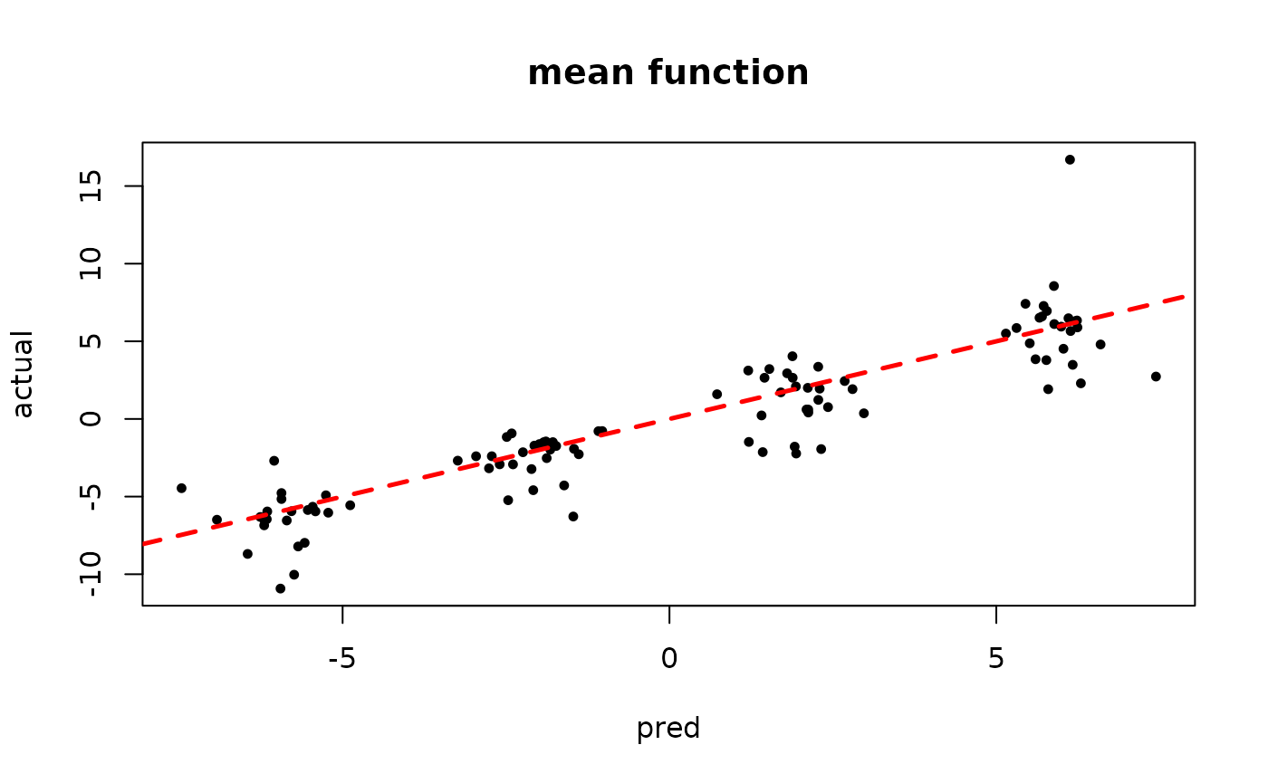

plot(rowMeans(bart_model_warmstart$sigma2_x_hat_test), s_x_test^2, 
     pch=16, cex=0.75, xlab = "pred", ylab = "actual", main = "variance function")
abline(0,1,col="red",lty=2,lwd=2.5)

MCMC

We now sample the $\sigma^2(X)$ ensemble using MCMC with root initialization (as in Chipman, George, and McCulloch (2010)).

num_gfr <- 0
num_burnin <- 1000
num_mcmc <- 100
num_samples <- num_gfr + num_burnin + num_mcmc
general_params <- list(sample_sigma2_global = F)
mean_forest_params <- list(sample_sigma2_leaf = F, num_trees = 50, 
                           alpha = 0.95, beta = 2, min_samples_leaf = 5)
variance_forest_params <- list(num_trees = 50, alpha = 0.95, 
                               beta = 1.25, min_samples_leaf = 5)
bart_model_mcmc <- stochtree::bart(
    X_train = X_train, y_train = y_train, X_test = X_test, 
    num_gfr = num_gfr, num_burnin = num_burnin, num_mcmc = num_mcmc, 
    general_params = general_params, mean_forest_params = mean_forest_params, 
    variance_forest_params = variance_forest_params
)

Inspect the MCMC samples

plot(rowMeans(bart_model_mcmc$y_hat_test), y_test, 
     pch=16, cex=0.75, xlab = "pred", ylab = "actual", main = "mean function")
abline(0,1,col="red",lty=2,lwd=2.5)

plot(rowMeans(bart_model_mcmc$sigma2_x_hat_test), s_x_test^2, 
     pch=16, cex=0.75, xlab = "pred", ylab = "actual", main = "variance function")
abline(0,1,col="red",lty=2,lwd=2.5)

Demo 4: Mean and Variance Simulation (complex DGP)

Simulation

Here, we generate data with more complex covariate-modified mean and variance functions.

$$\begin{equation*} \begin{aligned} y &= f(X) + \sigma(X) \epsilon\\ f(X) &= \begin{cases} -6X_4 & X_2 \geq 0 \text{ and } X_2 < 0.25\\ -2X_4 & X_2 \geq 0.25 \text{ and } X_2 < 0.5\\ 2X_4 & X_2 \geq 0.5 \text{ and } X_2 < 0.75\\ 6X_4 & X_2 \geq 0.75 \text{ and } X_2 < 1\\ \end{cases}\\ \sigma^2(X) &= \begin{cases} 0.25X_3^2 & X_1 \geq 0 \text{ and } X_1 < 0.25\\ 1X_3^2 & X_1 \geq 0.25 \text{ and } X_1 < 0.5\\ 4X_3^2 & X_1 \geq 0.5 \text{ and } X_1 < 0.75\\ 9X_3^2 & X_1 \geq 0.75 \text{ and } X_1 < 1\\ \end{cases}\\ X_1,\dots,X_p &\sim \text{U}\left(0,1\right)\\ \epsilon &\sim \mathcal{N}\left(0,1\right) \end{aligned} \end{equation*}$$

# Generate the data
n <- 500
p_x <- 10
X <- matrix(runif(n*p_x), ncol = p_x)
f_XW <- (
    ((0 <= X[,2]) & (0.25 > X[,2])) * (-6*X[,4]) + 
    ((0.25 <= X[,2]) & (0.5 > X[,2])) * (-2*X[,4]) + 
    ((0.5 <= X[,2]) & (0.75 > X[,2])) * (2*X[,4]) + 
    ((0.75 <= X[,2]) & (1 > X[,2])) * (6*X[,4])
)
s_XW <- (
    ((0 <= X[,1]) & (0.25 > X[,1])) * (0.5*X[,3]) + 
    ((0.25 <= X[,1]) & (0.5 > X[,1])) * (1*X[,3]) + 
    ((0.5 <= X[,1]) & (0.75 > X[,1])) * (2*X[,3]) + 
    ((0.75 <= X[,1]) & (1 > X[,1])) * (3*X[,3])
)
y <- f_XW + rnorm(n, 0, 1)*s_XW

# Split data into test and train sets
test_set_pct <- 0.2
n_test <- round(test_set_pct*n)
n_train <- n - n_test
test_inds <- sort(sample(1:n, n_test, replace = FALSE))
train_inds <- (1:n)[!((1:n) %in% test_inds)]
X_test <- as.data.frame(X[test_inds,])
X_train <- as.data.frame(X[train_inds,])
y_test <- y[test_inds]
y_train <- y[train_inds]
f_x_test <- f_XW[test_inds]
f_x_train <- f_XW[train_inds]
s_x_test <- s_XW[test_inds]
s_x_train <- s_XW[train_inds]

Sampling and Analysis

Warmstart

We first sample the $\sigma^2(X)$ ensemble using “warm-start” initialization (He and Hahn (2023)). This is the default in stochtree.

num_gfr <- 10
num_burnin <- 0
num_mcmc <- 100
num_samples <- num_gfr + num_burnin + num_mcmc
general_params <- list(sample_sigma2_global = F)
mean_forest_params <- list(sample_sigma2_leaf = F, num_trees = 50, 
                           alpha = 0.95, beta = 2, min_samples_leaf = 5)
variance_forest_params <- list(num_trees = 50, alpha = 0.95, 
                               beta = 1.25, min_samples_leaf = 5)
bart_model_warmstart <- stochtree::bart(
    X_train = X_train, y_train = y_train, X_test = X_test, 
    num_gfr = num_gfr, num_burnin = num_burnin, num_mcmc = num_mcmc, 
    general_params = general_params, mean_forest_params = mean_forest_params, 
    variance_forest_params = variance_forest_params
)

Inspect the MCMC samples

plot(rowMeans(bart_model_warmstart$y_hat_test), y_test, 
     pch=16, cex=0.75, xlab = "pred", ylab = "actual", main = "mean function")
abline(0,1,col="red",lty=2,lwd=2.5)

plot(rowMeans(bart_model_warmstart$sigma2_x_hat_test), s_x_test^2, 
     pch=16, cex=0.75, xlab = "pred", ylab = "actual", main = "variance function")
abline(0,1,col="red",lty=2,lwd=2.5)

MCMC

We now sample the $\sigma^2(X)$ ensemble using MCMC with root initialization (as in Chipman, George, and McCulloch (2010)).

num_gfr <- 0
num_burnin <- 1000
num_mcmc <- 100
num_samples <- num_gfr + num_burnin + num_mcmc
general_params <- list(sample_sigma2_global = F)
mean_forest_params <- list(sample_sigma2_leaf = F, num_trees = 50, 
                           alpha = 0.95, beta = 2, min_samples_leaf = 5)
variance_forest_params <- list(num_trees = 50, alpha = 0.95, 
                               beta = 1.25, min_samples_leaf = 5)
bart_model_mcmc <- stochtree::bart(
    X_train = X_train, y_train = y_train, X_test = X_test, 
    num_gfr = num_gfr, num_burnin = num_burnin, num_mcmc = num_mcmc, 
    general_params = general_params, mean_forest_params = mean_forest_params, 
    variance_forest_params = variance_forest_params
)

Inspect the MCMC samples

plot(rowMeans(bart_model_mcmc$y_hat_test), y_test, 
     pch=16, cex=0.75, xlab = "pred", ylab = "actual", main = "mean function")
abline(0,1,col="red",lty=2,lwd=2.5)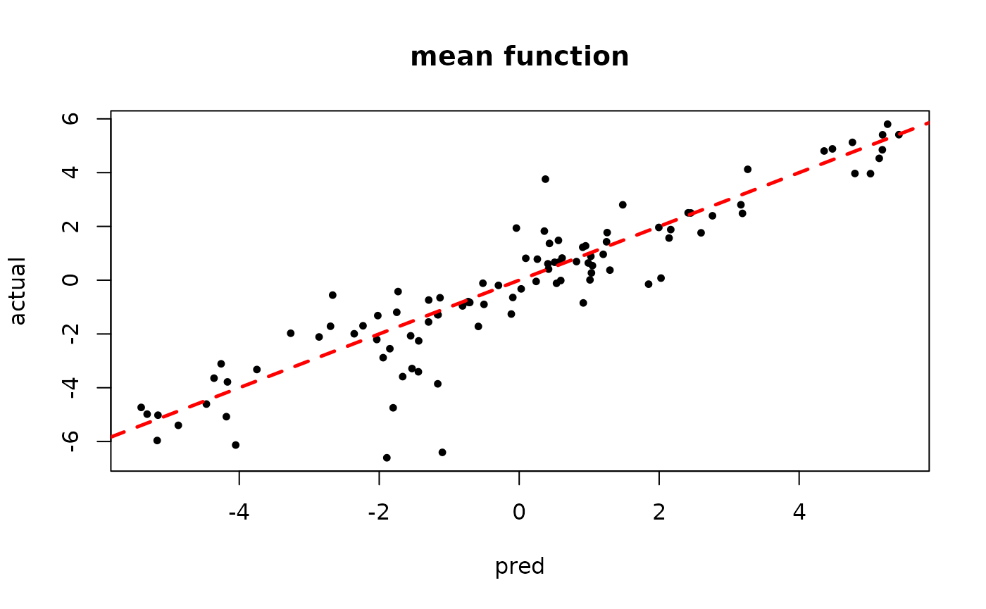

plot(rowMeans(bart_model_mcmc$sigma2_x_hat_test), s_x_test^2, 
     pch=16, cex=0.75, xlab = "pred", ylab = "actual", main = "variance function")
abline(0,1,col="red",lty=2,lwd=2.5)

Section 2: Causal Inference

Demo 1: Heterogeneous Treatment Effect, Continuous Treatment, Heteroskedastic Errors

We consider the following data generating process:

$$\begin{equation*} \begin{aligned} y &= \mu(X) + \tau(X) Z + \sigma(X) \epsilon\\ \sigma^2(X) &= \begin{cases} 0.25 & X_1 \geq 0 \text{ and } X_1 < 0.25\\ 1 & X_1 \geq 0.25 \text{ and } X_1 < 0.5\\ 4 & X_1 \geq 0.5 \text{ and } X_1 < 0.75\\ 9 & X_1 \geq 0.75 \text{ and } X_1 < 1\\ \end{cases}\\ \epsilon &\sim N\left(0,\sigma^2\right)\\ \mu(X) &= 1 + 2 X_1 - \mathbb{1}\left(X_2 < 0\right) \times 4 + \mathbb{1}\left(X_2 \geq 0\right) \times 4 + 3 \left(\lvert X_3 \rvert - \sqrt{\frac{2}{\pi}} \right)\\ \tau(X) &= 1 + 2 X_4\\ X_1,X_2,X_3,X_4,X_5 &\sim N\left(0,1\right)\\ U &\sim \text{Uniform}\left(0,1\right)\\ \pi(X) &= \frac{\mu(X) - 1}{2} + 4 \left(U - \frac{1}{2}\right)\\ Z &\sim \mathcal{N}\left(\pi(X), 1\right) \end{aligned} \end{equation*}$$

Simulation

We draw from the DGP defined above

n <- 2000
x1 <- rnorm(n)
x2 <- rnorm(n)
x3 <- rnorm(n)
x4 <- rnorm(n)
x5 <- rnorm(n)
X <- cbind(x1,x2,x3,x4,x5)
p <- ncol(X)
mu_x <- 1 + 2*x1 - 4*(x2 < 0) + 4*(x2 >= 0) + 3*(abs(x3) - sqrt(2/pi))
tau_x <- 1 + 2*x4
u <- runif(n)
pi_x <- ((mu_x-1)/4) + 4*(u-0.5)
Z <- pi_x + rnorm(n,0,1)
E_XZ <- mu_x + Z*tau_x
s_X <- (
    ((0 <= X[,1]) & (0.25 > X[,1])) * (0.5) + 
    ((0.25 <= X[,1]) & (0.5 > X[,1])) * (1) + 
    ((0.5 <= X[,1]) & (0.75 > X[,1])) * (2) + 
    ((0.75 <= X[,1]) & (1 > X[,1])) * (3)
)
y <- E_XZ + rnorm(n, 0, 1)*s_X
X <- as.data.frame(X)

# Split data into test and train sets
test_set_pct <- 0.2
n_test <- round(test_set_pct*n)
n_train <- n - n_test
test_inds <- sort(sample(1:n, n_test, replace = FALSE))
train_inds <- (1:n)[!((1:n) %in% test_inds)]
X_test <- X[test_inds,]
X_train <- X[train_inds,]
pi_test <- pi_x[test_inds]
pi_train <- pi_x[train_inds]
Z_test <- Z[test_inds]
Z_train <- Z[train_inds]
y_test <- y[test_inds]
y_train <- y[train_inds]
mu_test <- mu_x[test_inds]
mu_train <- mu_x[train_inds]
tau_test <- tau_x[test_inds]
tau_train <- tau_x[train_inds]
s_x_test <- s_X[test_inds]
s_x_train <- s_X[train_inds]

Sampling and Analysis

Warmstart

We first simulate from an ensemble model of $y \mid X$ using “warm-start” initialization samples (Krantsevich, He, and Hahn (2023)). This is the default in stochtree.

num_gfr <- 10
num_burnin <- 0
num_mcmc <- 100
num_samples <- num_gfr + num_burnin + num_mcmc
general_params <- list(keep_every = 5)
prognostic_forest_params <- list(sample_sigma2_leaf = F)
treatment_effect_forest_params <- list(sample_sigma2_leaf = F)
variance_forest_params <- list(num_trees = num_trees)
bcf_model_warmstart <- bcf(
    X_train = X_train, Z_train = Z_train, y_train = y_train, propensity_train = pi_train, 
    X_test = X_test, Z_test = Z_test, propensity_test = pi_test, 
    num_gfr = num_gfr, num_burnin = num_burnin, num_mcmc = num_mcmc, 
    general_params = general_params, prognostic_forest_params = prognostic_forest_params, 
    treatment_effect_forest_params = treatment_effect_forest_params, 
    variance_forest_params = variance_forest_params
)

Inspect the BART samples that were initialized with an XBART warm-start

plot(rowMeans(bcf_model_warmstart$mu_hat_test), mu_test, 
     xlab = "predicted", ylab = "actual", main = "Prognostic function")
abline(0,1,col="red",lty=3,lwd=3)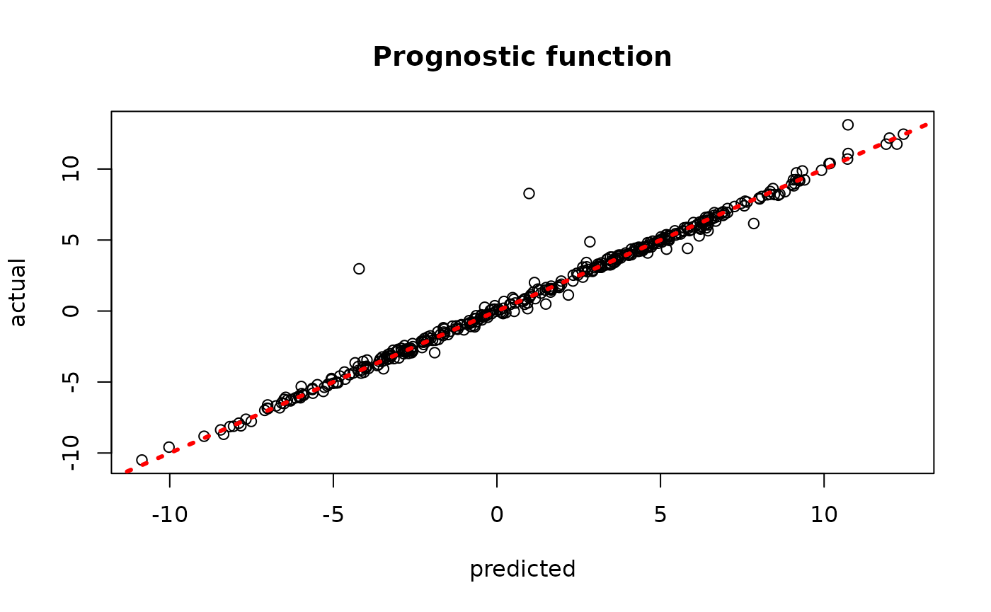

plot(rowMeans(bcf_model_warmstart$tau_hat_test), tau_test, 
     xlab = "predicted", ylab = "actual", main = "Treatment effect")
abline(0,1,col="red",lty=3,lwd=3)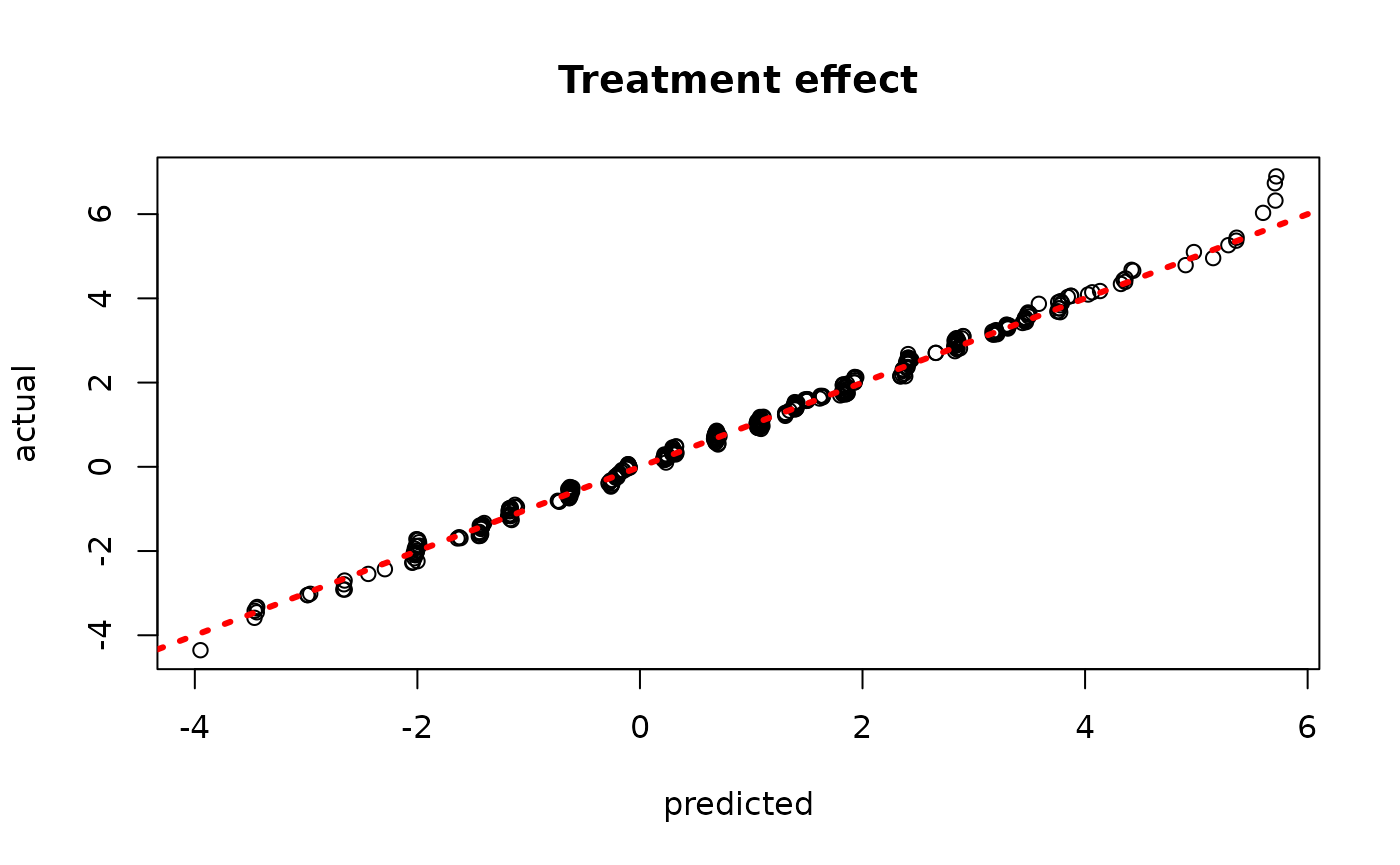

plot(rowMeans(bcf_model_warmstart$sigma2_x_hat_test), s_x_test^2, 
     pch=16, cex=0.75, xlab = "pred", ylab = "actual", main = "variance function")
abline(0,1,col="red",lty=2,lwd=2.5)

BART MCMC without Warmstart

Next, we simulate from this ensemble model without any warm-start initialization.

num_gfr <- 0
num_burnin <- 2000
num_mcmc <- 100
num_samples <- num_gfr + num_burnin + num_mcmc
general_params <- list(keep_every = 5)
prognostic_forest_params <- list(sample_sigma2_leaf = F)
treatment_effect_forest_params <- list(sample_sigma2_leaf = F)
variance_forest_params <- list(num_trees = num_trees)
bcf_model_root <- bcf(
    X_train = X_train, Z_train = Z_train, y_train = y_train, propensity_train = pi_train, 
    X_test = X_test, Z_test = Z_test, propensity_test = pi_test, 
    num_gfr = num_gfr, num_burnin = num_burnin, num_mcmc = num_mcmc, 
    general_params = general_params, prognostic_forest_params = prognostic_forest_params, 
    treatment_effect_forest_params = treatment_effect_forest_params, 
    variance_forest_params = variance_forest_params
)

Inspect the BART samples after burnin

plot(rowMeans(bcf_model_root$mu_hat_test), mu_test, 
     xlab = "predicted", ylab = "actual", main = "Prognostic function")
abline(0,1,col="red",lty=3,lwd=3)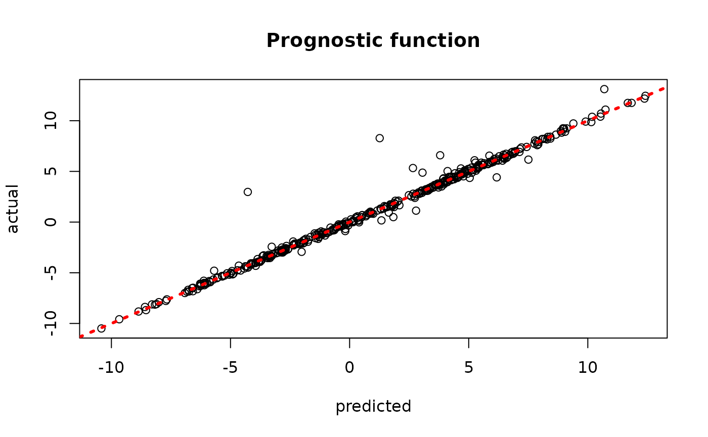

plot(rowMeans(bcf_model_root$tau_hat_test), tau_test, 
     xlab = "predicted", ylab = "actual", main = "Treatment effect")
abline(0,1,col="red",lty=3,lwd=3)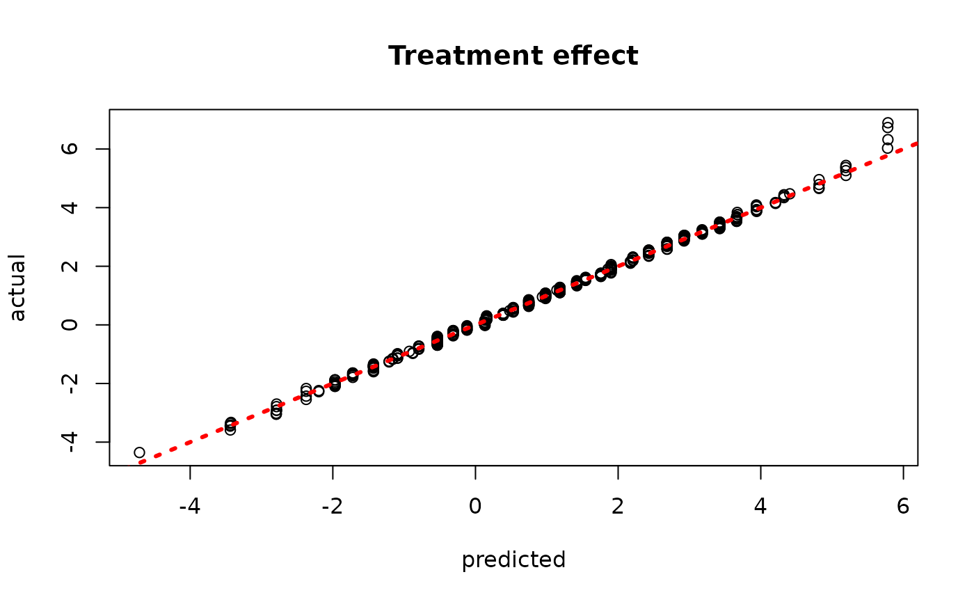

plot(rowMeans(bcf_model_root$sigma2_x_hat_test), s_x_test^2, 
     pch=16, cex=0.75, xlab = "pred", ylab = "actual", main = "variance function")
abline(0,1,col="red",lty=2,lwd=2.5)

References

Chipman, Hugh A., Edward I. George, and Robert E. McCulloch. 2010. “BART: Bayesian additive regression trees.” The Annals of Applied Statistics 4 (1): 266–98. https://doi.org/10.1214/09-AOAS285.

Hahn, P Richard, Jared S Murray, and Carlos M Carvalho. 2020. “Bayesian Regression Tree Models for Causal Inference: Regularization, Confounding, and Heterogeneous Effects (with Discussion).” Bayesian Analysis 15 (3): 965–1056.

He, Jingyu, and P Richard Hahn. 2023. “Stochastic Tree Ensembles for Regularized Nonlinear Regression.” Journal of the American Statistical Association 118 (541): 551–70.

Krantsevich, Nikolay, Jingyu He, and P Richard Hahn. 2023. “Stochastic Tree Ensembles for Estimating Heterogeneous Effects.” In International Conference on Artificial Intelligence and Statistics, 6120–31. PMLR.

Murray, Jared S. 2021. “Log-Linear Bayesian Additive Regression Trees for Multinomial Logistic and Count Regression Models.” Journal of the American Statistical Association 116 (534): 756–69.