Summary and Plotting Utilities • stochtree

This vignette demonstrates the summary and plotting utilities available for stochtree models in R.

To begin, we load the stochtree package.

library(stochtree)

and set a random seed for reproducibility.

random_seed = 1234
set.seed(random_seed)

Supervised Learning

We begin with the supervised learning use case served by the bart() function.

Below we simulate a simple regression dataset.

n <- 1000
p_x <- 10
p_w <- 1
X <- matrix(runif(n * p_x), ncol = p_x)
W <- matrix(runif(n * p_w), ncol = p_w)
f_XW <- (((0 <= X[, 10]) & (0.25 > X[, 10])) *
  (-7.5 * W[, 1]) +
  ((0.25 <= X[, 10]) & (0.5 > X[, 10])) * (-2.5 * W[, 1]) +
  ((0.5 <= X[, 10]) & (0.75 > X[, 10])) * (2.5 * W[, 1]) +
  ((0.75 <= X[, 10]) & (1 > X[, 10])) * (7.5 * W[, 1]))
noise_sd <- 1
y <- f_XW + rnorm(n, 0, 1) * noise_sd

Now we fit a simple BART model to the data

num_gfr <- 10
num_burnin <- 0
num_mcmc <- 1000
general_params <- list(num_chains = 3)
bart_model <- stochtree::bart(
  X_train = X,
  y_train = y,
  leaf_basis_train = W,
  num_gfr = num_gfr,
  num_burnin = num_burnin,
  num_mcmc = num_mcmc,
  general_params = general_params
)

We obtain a high level summary of the BART model by running print()

print(bart_model)
#> stochtree::bart() run with mean forest, global error variance model, and mean forest leaf scale model
#> Continuous outcome was modeled as Gaussian with a leaf regression prior with 1 bases for the mean forest
#> Outcome was standardized
#> The sampler was run for 10 GFR iterations, with 3 chains of 0 burn-in iterations and 1000 MCMC iterations, retaining every iteration (i.e. no thinning)

For a more detailed summary (including the information above), we use the summary() function.

summary(bart_model)
#> stochtree::bart() run with mean forest, global error variance model, and mean forest leaf scale model
#> Continuous outcome was modeled as Gaussian with a leaf regression prior with 1 bases for the mean forest
#> Outcome was standardized
#> The sampler was run for 10 GFR iterations, with 3 chains of 0 burn-in iterations and 1000 MCMC iterations, retaining every iteration (i.e. no thinning) 
#> Summary of sigma^2 posterior: 
#> 3000 samples, mean = 0.888, standard deviation = 0.047, quantiles:
#>      2.5%       10%       25%       50%       75%       90%     97.5% 
#> 0.8005121 0.8278741 0.8547766 0.8867185 0.9188729 0.9499080 0.9814877 
#> Summary of leaf scale posterior: 
#> 3000 samples, mean = 0.007, standard deviation = 0.001, quantiles:
#>        2.5%         10%         25%         50%         75%         90% 
#> 0.005066028 0.005522443 0.006119807 0.006790362 0.007601055 0.008540178 
#>       97.5% 
#> 0.009936252 
#> Summary of in-sample posterior mean predictions: 
#> 1000 observations, mean = -0.064, standard deviation = 3.285, quantiles:
#>      2.5%       10%       25%       50%       75%       90%     97.5% 
#> -6.852160 -4.925664 -1.818674 -0.114368  2.002915  4.300611  6.522902

We can use the plot() function to produce a traceplot of model terms like the global error scale $\sigma^2$ or (if $\sigma^2$ is not sampled) the first observation of cached train set predictions

plot(bart_model)

For finer-grained control over which parameters to plot, we can also use the extract_parameter() function to pull the posterior distribution of any valid model term (e.g., global error scale $\sigma^2$ , leaf scale $\sigma^2_{\ell}$ , in-sample mean function predictions y_hat_train) and then plot any subset or transformation of these values.

y_hat_train_samples <- extract_parameter(bart_model, "y_hat_train")
obs_index <- 1
plot(
  y_hat_train_samples[obs_index, ],
  type = "l",
  main = paste0("In-Sample Predictions Traceplot, Observation ", obs_index),
  xlab = "Index",
  ylab = "Parameter Values"
)

Causal Inference

We now run the same demo for the causal inference use case served by the bcf() function.

Below we simulate a simple dataset for a causal inference problem with binary treatment and continuous outcome.

# Generate covariates and treatment
n <- 1000
p_X = 5
X = matrix(runif(n * p_X), ncol = p_X)
pi_X = 0.25 + 0.5 * X[, 1]
Z = rbinom(n, 1, pi_X)

# Define the outcome mean functions (prognostic and treatment effects)
mu_X = pi_X * 5 + 2 * X[, 3]
tau_X = X[, 2] * 2 - 1

# Generate outcome
epsilon = rnorm(n, 0, 1)
y = mu_X + tau_X * Z + epsilon

Now we fit a simple BCF model to the data

num_gfr <- 10
num_burnin <- 0
num_mcmc <- 1000
general_params <- list(num_chains = 3)
bcf_model <- stochtree::bcf(
  X_train = X,
  y_train = y,
  Z_train = Z,
  num_gfr = num_gfr,
  num_burnin = num_burnin,
  num_mcmc = num_mcmc,
  general_params = general_params
)

We obtain a high level summary of the BCF model by running print()

print(bcf_model)
#> stochtree::bcf() run with prognostic forest, treatment effect forest, global error variance model, and prognostic forest leaf scale model
#> Outcome was modeled as gaussian
#> Treatment was binary and its effect was estimated with adaptive coding
#> outcome was standardized
#> An internal propensity model was fit using stochtree::bart() in lieu of user-provided propensity scores
#> The sampler was run for 10 GFR iterations, with 3 chains of 0 burn-in iterations and 1000 MCMC iterations, retaining every iteration (i.e. no thinning)

For a more detailed summary (including the information above), we use the summary() function.

summary(bcf_model)
#> stochtree::bcf() run with prognostic forest, treatment effect forest, global error variance model, and prognostic forest leaf scale model
#> Outcome was modeled as gaussian
#> Treatment was binary and its effect was estimated with adaptive coding
#> outcome was standardized
#> An internal propensity model was fit using stochtree::bart() in lieu of user-provided propensity scores
#> The sampler was run for 10 GFR iterations, with 3 chains of 0 burn-in iterations and 1000 MCMC iterations, retaining every iteration (i.e. no thinning) 
#> Summary of sigma^2 posterior: 
#> 3000 samples, mean = 0.953, standard deviation = 0.046, quantiles:
#>      2.5%       10%       25%       50%       75%       90%     97.5% 
#> 0.8687535 0.8959173 0.9226951 0.9518836 0.9814306 1.0129240 1.0492748 
#> Summary of prognostic forest leaf scale posterior: 
#> 3000 samples, mean = 0.001, standard deviation = 0.000, quantiles:
#>         2.5%          10%          25%          50%          75%          90% 
#> 0.0008736919 0.0010011085 0.0011354539 0.0013164351 0.0015554243 0.0017913780 
#>        97.5% 
#> 0.0021597952 
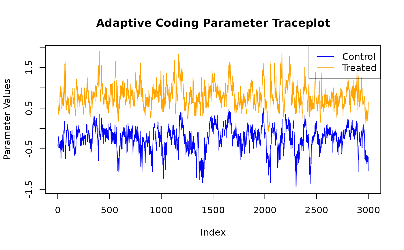
#> Summary of adaptive coding parameters: 
#> 3000 samples, mean (control) = -0.252, mean (treated) = 0.799, standard deviation (control) = 0.291, standard deviation (treated) = 0.280
#> quantiles (control):
#>        2.5%         10%         25%         50%         75%         90% 
#> -0.97717823 -0.64351472 -0.40129570 -0.22008660 -0.06046424  0.07960515 
#>       97.5% 
#>  0.23481890 
#> quantiles (treated):
#>      2.5%       10%       25%       50%       75%       90%     97.5% 
#> 0.3050494 0.4800757 0.6089559 0.7763713 0.9574100 1.1731817 1.4447201 
#> Summary of in-sample posterior mean predictions: 
#> 1000 observations, mean = 3.488, standard deviation = 0.941, quantiles:
#>     2.5%      10%      25%      50%      75%      90%    97.5% 
#> 1.691197 2.269548 2.814026 3.473908 4.116115 4.721470 5.427572 
#> Summary of in-sample posterior mean CATEs: 
#> 1000 observations, mean = 0.077, standard deviation = 0.529, quantiles:
#>        2.5%         10%         25%         50%         75%         90% 
#> -0.70303416 -0.55178665 -0.39842320 -0.01740183  0.61660477  0.78620384 
#>       97.5% 
#>  0.88377780

We can use the plot() function to produce a traceplot of model terms like the global error scale $\sigma^2$ or (if $\sigma^2$ is not sampled) the first observation of cached train set predictions

plot(bcf_model)

For finer-grained control over which parameters to plot, we can also use the extract_parameter() function to pull the posterior distribution of any valid model term (e.g., global error scale $\sigma^2$ , prognostic forest leaf scale $\sigma^2_{\mu}$ , CATE forest leaf scale $\sigma^2_{\tau}$ , adaptive coding parameters $b_0$ and $b_1$ for binary treatment, in-sample mean function predictions y_hat_train, in-sample CATE function predictions tau_hat_train) and then plot any subset or transformation of these values.

adaptive_coding_samples <- extract_parameter(bcf_model, "adaptive_coding")
plot(
  adaptive_coding_samples[1, ],
  type = "l",
  main = "Adaptive Coding Parameter Traceplot",
  xlab = "Index",
  ylab = "Parameter Values",
  ylim = range(adaptive_coding_samples),
  col = "blue"
)
lines(adaptive_coding_samples[2, ], col = "orange")
legend(
  "topright",
  legend = c("Control", "Treated"),
  lty = 1,
  col = c("blue", "orange")
)