Semiparametric Causal Inference in StochTree

The classic BCF model of Hahn, Murray, and Carvalho (2020) is defined as $$\begin{equation} \begin{aligned} Y_i \mid x_i, z_i &\sim \mathrm{N}(f_0(x_i) + \tau(x_i) z_i, \sigma^2)\\ f_0 &\sim \mathrm{BART}(\alpha_0, \beta_0, m_0)\\ \tau &\sim \mathrm{BART}(\alpha_{\tau}, \beta_{\tau}, m_{\tau}). \end{aligned} \end{equation}$$ where $\mathrm{BART}(\alpha, \beta, m)$ defines a BART model with $m$ trees and split prior parameters $\alpha$ and $\beta$.

The authors noted that separating estimation / regularization of a control function, $f_0(x)$, and a CATE function, $\tau(x)$, can give better estimation error and interval coverage in settings with strong confounding and treatment effect moderation.

stochtree now defaults to a slight modification of this model, with the treatment effect function decomposed into parametric and nonparametric components $$\begin{equation} \begin{aligned} Y_i \mid x_i, z_i &\sim \mathrm{N}(f_0(x_i) + (\tau_0 + t(x_i)) z_i, \sigma^2)\\ f_0 &\sim \mathrm{BART}(\alpha_0, \beta_0, m_0)\\ t &\sim \mathrm{BART}(\alpha_{t}, \beta_{t}, m_{t})\\ \tau_0 &\sim \mathrm{N}\left(0, \sigma_{\tau_0}^2 \right), \end{aligned} \end{equation}$$ where $\tau_0 + t(x_i)$ takes the place of the $\tau(x_i)$ forest term in the original BCF model. This decomposition allows the forest term to focus on capturing heterogeneity “offsets” to a parametric model of homogeneous treatment effects.

Below we demonstrate the advantages of this “reparameterization” of BCF on a synthetic dataset.

First, we load the necessary libraries

library(stochtree)

We set a seed for reproducibility

random_seed <- 1234
set.seed(random_seed)

Binary Treatment with Homogeneous Treatment Effect

Consider the following data generating process

$$\begin{equation*} \begin{aligned} y &= \mu(X) + \tau(X) Z + \epsilon\\ \mu(X) &= 2 \sin(2 \pi X_1) - 2 (2 X_3 - 1)\\ \tau(X) &= 5\\ \pi(X) &= \phi\left(\frac{\mu(X)}{4}\right)\\ X_1,\dots,X_p &\sim \text{Uniform}\left(0,1\right)\\ Z &\sim \text{Bernoulli}\left(\pi(X)\right)\\ \epsilon &\sim N\left(0,\sigma^2\right) \end{aligned} \end{equation*}$$

Simulation

We draw from the DGP defined above

n <- 500
p <- 20
snr <- 2
X <- matrix(runif(n * p), n, p)
mu_x <- 2 * sin(2 * pi * X[, 1]) - 2 * (2 * X[, 3] - 1)
tau_x <- 5
pi_x <- pnorm(mu_x / 4)
Z <- rbinom(n, 1, pi_x)
E_XZ <- mu_x + Z * tau_x
sigma_true <- sd(E_XZ) / snr
y <- E_XZ + rnorm(n, 0, 1) * sigma_true

And split data into test and train sets

test_set_pct <- 0.5
n_test <- round(test_set_pct * n)
n_train <- n - n_test
test_inds <- sort(sample(1:n, n_test, replace = FALSE))
train_inds <- (1:n)[!((1:n) %in% test_inds)]
X_test <- X[test_inds, ]
X_train <- X[train_inds, ]
pi_test <- pi_x[test_inds]
pi_train <- pi_x[train_inds]
Z_test <- Z[test_inds]
Z_train <- Z[train_inds]
y_test <- y[test_inds]
y_train <- y[train_inds]
mu_test <- mu_x[test_inds]
mu_train <- mu_x[train_inds]
tau_test <- tau_x[test_inds]
tau_train <- tau_x[train_inds]

Sampling and Analysis

Classic BCF Model

We first simulate from the classic BCF model with no parametric treatment effect term

num_gfr <- 0
num_burnin <- 1000
num_mcmc <- 500
general_params <- list(
  adaptive_coding = TRUE,
  num_chains = 4,
  random_seed = random_seed,
  num_threads = 1
)
num_trees_tau <- 50
treatment_effect_forest_params <- list(
  num_trees = num_trees_tau,
  sample_intercept = FALSE,
  sigma2_leaf_init = 1 / num_trees_tau
)
bcf_model_classic <- bcf(
  X_train = X_train,
  Z_train = Z_train,
  y_train = y_train,
  propensity_train = pi_train,
  X_test = X_test,
  Z_test = Z_test,
  propensity_test = pi_test,
  num_gfr = num_gfr,
  num_burnin = num_burnin,
  num_mcmc = num_mcmc,
  general_params = general_params,
  treatment_effect_forest_params = treatment_effect_forest_params
)

And we compare the posterior distribution of the ATE to its true value

cate_posterior_classic <- predict(
  bcf_model_classic,
  X = X_test,
  Z = Z_test,
  propensity = pi_test,
  type = "posterior",
  terms = "cate"
)
ate_posterior_classic <- colMeans(cate_posterior_classic)
hist(
  ate_posterior_classic,
  freq = F,
  xlab = "ATE",
  ylab = "Density",
  main = "Posterior Distribution of ATE"
)
abline(v = tau_x, col = "red", lty = 3, lwd = 3)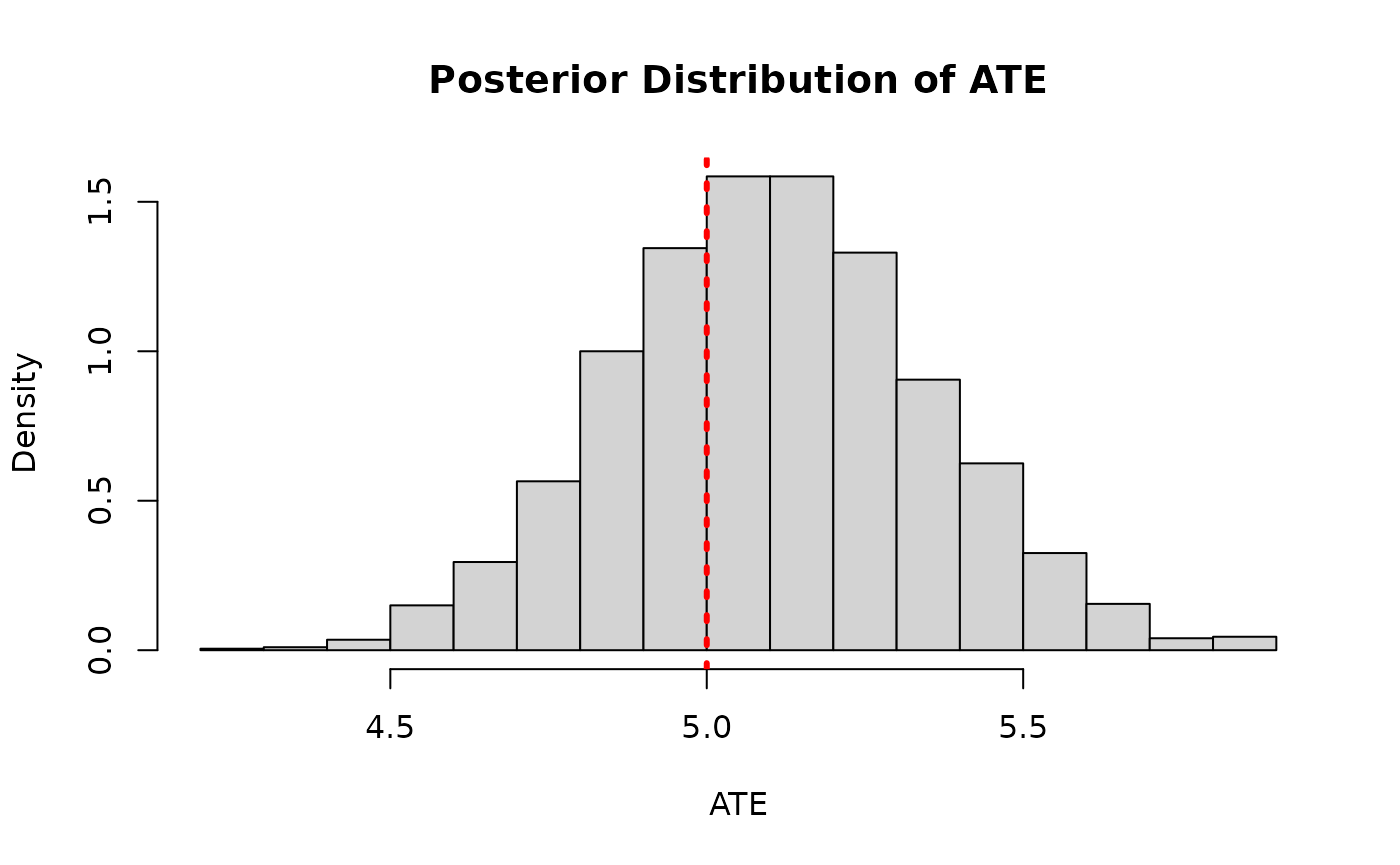

As a rough convergence check, we inspect the traceplot of the global error scale parameter, $\sigma^2$

sigma2_samples <- extractParameter(bcf_model_classic, "sigma2")
plot(
  sigma2_samples,
  type = "l",
  main = "Traceplot of Sigma^2",
  ylab = "Sigma^2",
  xlab = "Iteration"
)
abline(h = sigma_true^2, col = "red", lty = 3, lwd = 3)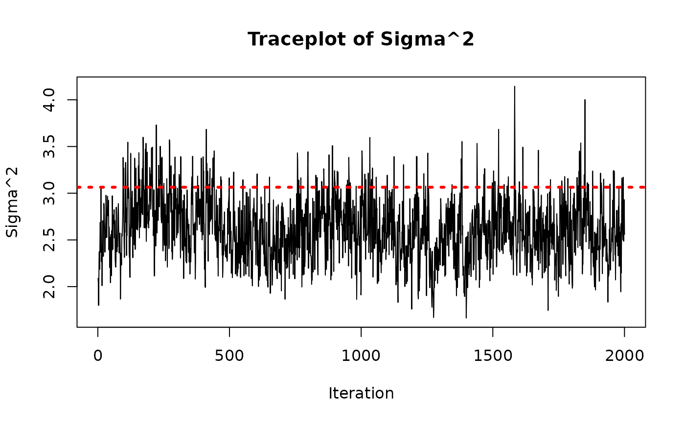

Reparameterized BCF Model

Now we fit the reparameterized model, regularizing the $t(x)$ forest more heavily to account for the standard normal prior on the $\tau_0$ term.

num_trees_tau <- 50
general_params <- list(
  adaptive_coding = FALSE,
  num_chains = 4,
  random_seed = random_seed,
  num_threads = 1
)
treatment_effect_forest_params <- list(
  num_trees = num_trees_tau,
  sample_intercept = TRUE,
  sigma2_leaf_init = 0.25 / num_trees_tau,
  tau_0_prior_var = 1
)
bcf_model_reparam <- bcf(
  X_train = X_train,
  Z_train = Z_train,
  y_train = y_train,
  propensity_train = pi_train,
  X_test = X_test,
  Z_test = Z_test,
  propensity_test = pi_test,
  num_gfr = num_gfr,
  num_burnin = num_burnin,
  num_mcmc = num_mcmc,
  general_params = general_params,
  treatment_effect_forest_params = treatment_effect_forest_params
)

And we compare the posterior distribution of the ATE to its true value

cate_posterior_reparam <- predict(
  bcf_model_reparam,
  X = X_test,
  Z = Z_test,
  propensity = pi_test,
  type = "posterior",
  terms = "cate"
)
ate_posterior_reparam <- colMeans(cate_posterior_reparam)
hist(
  ate_posterior_reparam,
  freq = F,
  xlab = "ATE",
  ylab = "Density",
  main = "Posterior Distribution of ATE"
)
abline(v = tau_x, col = "red", lty = 3, lwd = 3)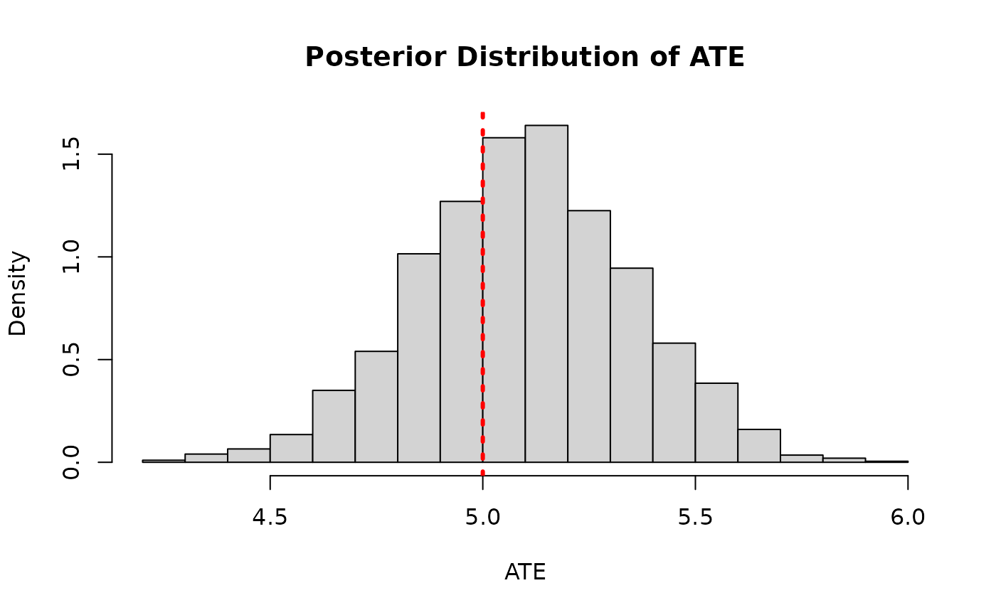

As above, we check convergence by inspecting the traceplot of the global error scale parameter, $\sigma^2$

sigma2_samples <- extractParameter(bcf_model_reparam, "sigma2")
plot(
  sigma2_samples,
  type = "l",
  main = "Traceplot of Sigma^2",
  ylab = "Sigma^2",
  xlab = "Iteration"
)
abline(h = sigma_true^2, col = "red", lty = 3, lwd = 3)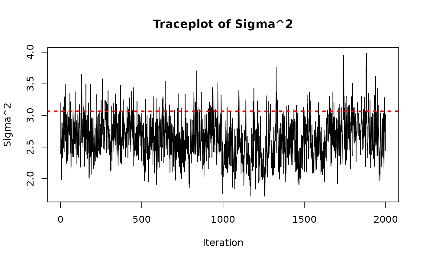

Since $t(X)$ is not constrained to sum to 0, the parameter $\tau_0$ does not identify the ATE. We can see this by averaging each posterior draw of $t(X)$ over the test set and comparing the posterior point estimates $\tau_0$ and $\bar{t}(X)$.

tau_0_posterior <- extractParameter(bcf_model_reparam, "tau_0")
t_x_posterior_reparam <- predict(
  bcf_model_reparam,
  X = X_test,
  Z = Z_test,
  propensity = pi_test,
  type = "posterior",
  terms = "tau"
)
t_x_posterior_reparam <- colMeans(t_x_posterior_reparam)
plot(
  tau_0_posterior,
  t_x_posterior_reparam,
  xlab = "tau_0",
  ylab = "t(X)",
  main = "Posterior of tau_0 vs t(X), averaged over X"
)

While stochtree does not currently support constraining $t(X)$ to sum to 0 over the training set, we can more heavily regularize $t(X)$ so that its values are much closer to zero. Using a single tree with a very small leaf scale effectively collapses the forest to a constant near zero, making $\tau_0$ the primary vehicle for the treatment effect.

general_params <- list(
  adaptive_coding = FALSE,
  num_chains = 4,
  random_seed = random_seed,
  num_threads = 1
)
treatment_effect_forest_params <- list(
  num_trees = 1,
  sample_intercept = TRUE,
  sigma2_leaf_init = 1e-6,
  tau_0_prior_var = 1
)
bcf_model_reparam <- bcf(
  X_train = X_train,
  Z_train = Z_train,
  y_train = y_train,
  propensity_train = pi_train,
  X_test = X_test,
  Z_test = Z_test,
  propensity_test = pi_test,
  num_gfr = num_gfr,
  num_burnin = num_burnin,
  num_mcmc = num_mcmc,
  general_params = general_params,
  treatment_effect_forest_params = treatment_effect_forest_params
)

Again we plot the posterior distribution of the ATE

cate_posterior_reparam <- predict(
  bcf_model_reparam,
  X = X_test,
  Z = Z_test,
  propensity = pi_test,
  type = "posterior",
  terms = "cate"
)
ate_posterior_reparam <- colMeans(cate_posterior_reparam)
hist(
  ate_posterior_reparam,
  freq = F,
  xlab = "ATE",
  ylab = "Density",
  main = "Posterior Distribution of ATE"
)
abline(v = tau_x, col = "red", lty = 3, lwd = 3)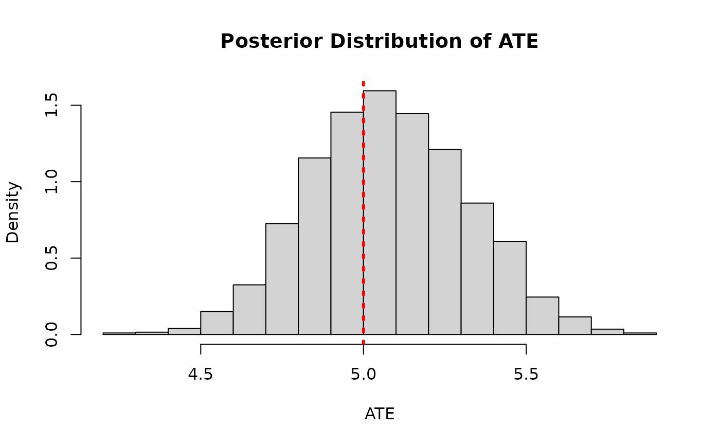

This time we see no correlation between the $\tau_0$ posterior and the (highly-regularized) $\bar{t}(X)$ posterior – $\tau_0$ more directly captures the majority of the ATE

tau_0_posterior <- extractParameter(bcf_model_reparam, "tau_0")
t_x_posterior_reparam <- predict(
  bcf_model_reparam,
  X = X_test,
  Z = Z_test,
  propensity = pi_test,
  type = "posterior",
  terms = "tau"
)
t_x_posterior_reparam <- colMeans(t_x_posterior_reparam)
plot(
  tau_0_posterior,
  t_x_posterior_reparam,
  xlab = "tau_0",
  ylab = "t(X)",
  main = "Posterior of tau_0 vs t(X), averaged over X"
)
abline(0, 1, col = "red", lty = 3, lwd = 3)

We can further regularize estimation of the ATE by reducing $\sigma_{\tau_0}^2$

general_params <- list(
  adaptive_coding = FALSE,
  num_chains = 4,
  random_seed = random_seed,
  num_threads = 1
)
treatment_effect_forest_params <- list(
  num_trees = 1,
  sample_intercept = TRUE,
  sigma2_leaf_init = 1e-6,
  tau_0_prior_var = 0.05
)
bcf_model_reparam <- bcf(
  X_train = X_train,
  Z_train = Z_train,
  y_train = y_train,
  propensity_train = pi_train,
  X_test = X_test,
  Z_test = Z_test,
  propensity_test = pi_test,
  num_gfr = num_gfr,
  num_burnin = num_burnin,
  num_mcmc = num_mcmc,
  general_params = general_params,
  treatment_effect_forest_params = treatment_effect_forest_params
)
cate_posterior_reparam <- predict(
  bcf_model_reparam,
  X = X_test,
  Z = Z_test,
  propensity = pi_test,
  type = "posterior",
  terms = "cate"
)
ate_posterior_reparam <- colMeans(cate_posterior_reparam)
hist(
  ate_posterior_reparam,
  freq = F,
  xlab = "ATE",
  ylab = "Density",
  main = "Posterior Distribution of ATE"
)
abline(v = tau_x, col = "red", lty = 3, lwd = 3)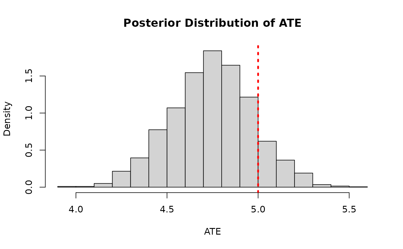

Continuous Treatment with Homogeneous Treatment Effect

The $\tau_0 + t(x)$ reparameterization generalizes naturally to continuous treatment. With a continuous $Z$, $\tau(x)$ represents the marginal effect of a one-unit increase in $Z$, and $\tau_0$ captures the homogeneous component of that effect.

Consider the following data generating process:

$$\begin{equation*} \begin{aligned} y &= \mu(X) + \tau(X)\, Z + \epsilon\\ \mu(X) &= 2 \sin(2 \pi X_1) - 2 (2 X_3 - 1)\\ \tau(X) &= 2\\ \pi(X) &= \mathrm{E}[Z \mid X] = \mu(X)/8\\ Z \mid X &\sim \mathrm{N}(\pi(X),\, 1)\\ \epsilon &\sim N\left(0,\sigma^2\right) \end{aligned} \end{equation*}$$

Simulation

We draw from the DGP defined above

n <- 500
p <- 20
snr <- 2
X <- matrix(runif(n * p), n, p)
mu_x <- 2 * sin(2 * pi * X[, 1]) - 2 * (2 * X[, 3] - 1)
tau_x <- 2
pi_x <- mu_x / 8
Z <- pi_x + rnorm(n, 0, 1)
E_XZ <- mu_x + Z * tau_x
sigma_true <- sd(E_XZ) / snr
y <- E_XZ + rnorm(n, 0, 1) * sigma_true

And split data into test and train sets

test_inds <- sort(sample(1:n, round(0.5 * n), replace = FALSE))
train_inds <- (1:n)[!((1:n) %in% test_inds)]
X_test <- X[test_inds, ]
X_train <- X[train_inds, ]
pi_test <- pi_x[test_inds]
pi_train <- pi_x[train_inds]
Z_test <- Z[test_inds]
Z_train <- Z[train_inds]
y_test <- y[test_inds]
y_train <- y[train_inds]

Sampling and Analysis

Note that adaptive_coding must be FALSE for continuous treatment, since the adaptive coding scheme is designed for binary treatment.

Classic BCF Model

num_gfr <- 0
num_burnin <- 1000
num_mcmc <- 500
general_params <- list(
  adaptive_coding = FALSE,
  num_chains = 4,
  random_seed = random_seed,
  num_threads = 1
)
num_trees_tau <- 50
treatment_effect_forest_params <- list(
  num_trees = num_trees_tau,
  sample_intercept = FALSE,
  sigma2_leaf_init = 1 / num_trees_tau
)
bcf_model_classic <- bcf(
  X_train = X_train,
  Z_train = Z_train,
  y_train = y_train,
  propensity_train = pi_train,
  X_test = X_test,
  Z_test = Z_test,
  propensity_test = pi_test,
  num_gfr = num_gfr,
  num_burnin = num_burnin,
  num_mcmc = num_mcmc,
  general_params = general_params,
  treatment_effect_forest_params = treatment_effect_forest_params
)

We compare the posterior distribution of the ATE to its true value

cate_posterior_classic <- predict(
  bcf_model_classic,
  X = X_test,
  Z = Z_test,
  propensity = pi_test,
  type = "posterior",
  terms = "cate"
)
ate_posterior_classic <- colMeans(cate_posterior_classic)
hist(
  ate_posterior_classic,
  freq = F,
  xlab = "ATE",
  ylab = "Density",
  main = "Posterior Distribution of ATE (Classic BCF, Continuous Treatment)"
)
abline(v = tau_x, col = "red", lty = 3, lwd = 3)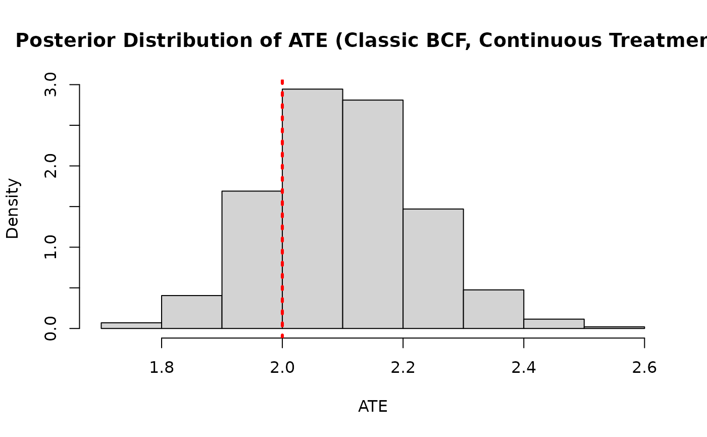

As a rough convergence check, we inspect the traceplot of $\sigma^2$

sigma2_samples <- extractParameter(bcf_model_classic, "sigma2")
plot(
  sigma2_samples,
  type = "l",
  main = "Traceplot of Sigma^2 (Classic BCF, Continuous Treatment)",
  ylab = "Sigma^2",
  xlab = "Iteration"
)
abline(h = sigma_true^2, col = "red", lty = 3, lwd = 3)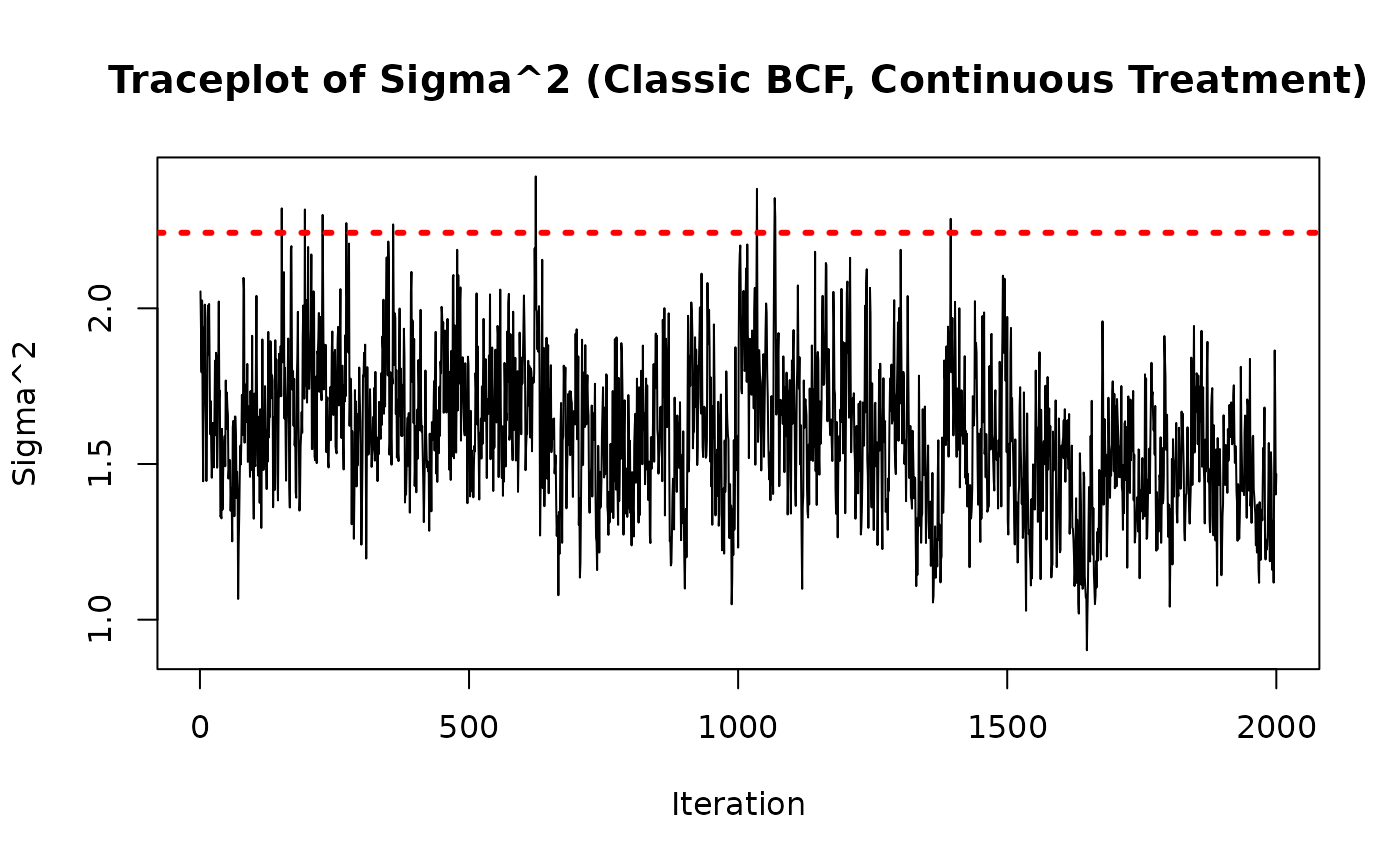

Reparameterized BCF Model

treatment_effect_forest_params <- list(
  num_trees = num_trees_tau,
  sample_intercept = TRUE,
  sigma2_leaf_init = 0.25 / num_trees_tau,
  tau_0_prior_var = 1
)
bcf_model_reparam <- bcf(
  X_train = X_train,
  Z_train = Z_train,
  y_train = y_train,
  propensity_train = pi_train,
  X_test = X_test,
  Z_test = Z_test,
  propensity_test = pi_test,
  num_gfr = num_gfr,
  num_burnin = num_burnin,
  num_mcmc = num_mcmc,
  general_params = general_params,
  treatment_effect_forest_params = treatment_effect_forest_params
)

And we compare the posterior distribution of the ATE to its true value

cate_posterior_reparam <- predict(
  bcf_model_reparam,
  X = X_test,
  Z = Z_test,
  propensity = pi_test,
  type = "posterior",
  terms = "cate"
)
ate_posterior_reparam <- colMeans(cate_posterior_reparam)
hist(
  ate_posterior_reparam,
  freq = F,
  xlab = "ATE",
  ylab = "Density",
  main = "Posterior Distribution of ATE (Reparameterized BCF, Continuous Treatment)"
)
abline(v = tau_x, col = "red", lty = 3, lwd = 3)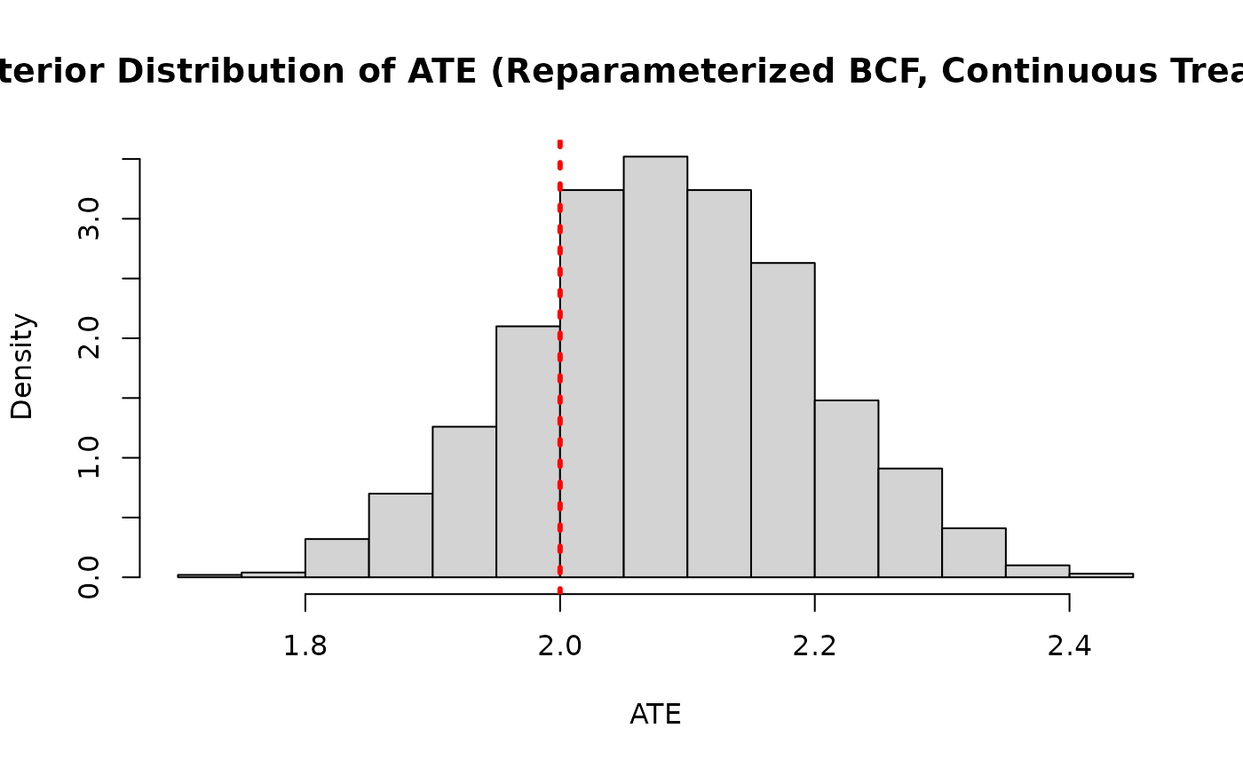

As above, we check convergence by inspecting the traceplot of $\sigma^2$

sigma2_samples <- extractParameter(bcf_model_reparam, "sigma2")
plot(
  sigma2_samples,
  type = "l",
  main = "Traceplot of Sigma^2 (Reparameterized BCF, Continuous Treatment)",
  ylab = "Sigma^2",
  xlab = "Iteration"
)
abline(h = sigma_true^2, col = "red", lty = 3, lwd = 3)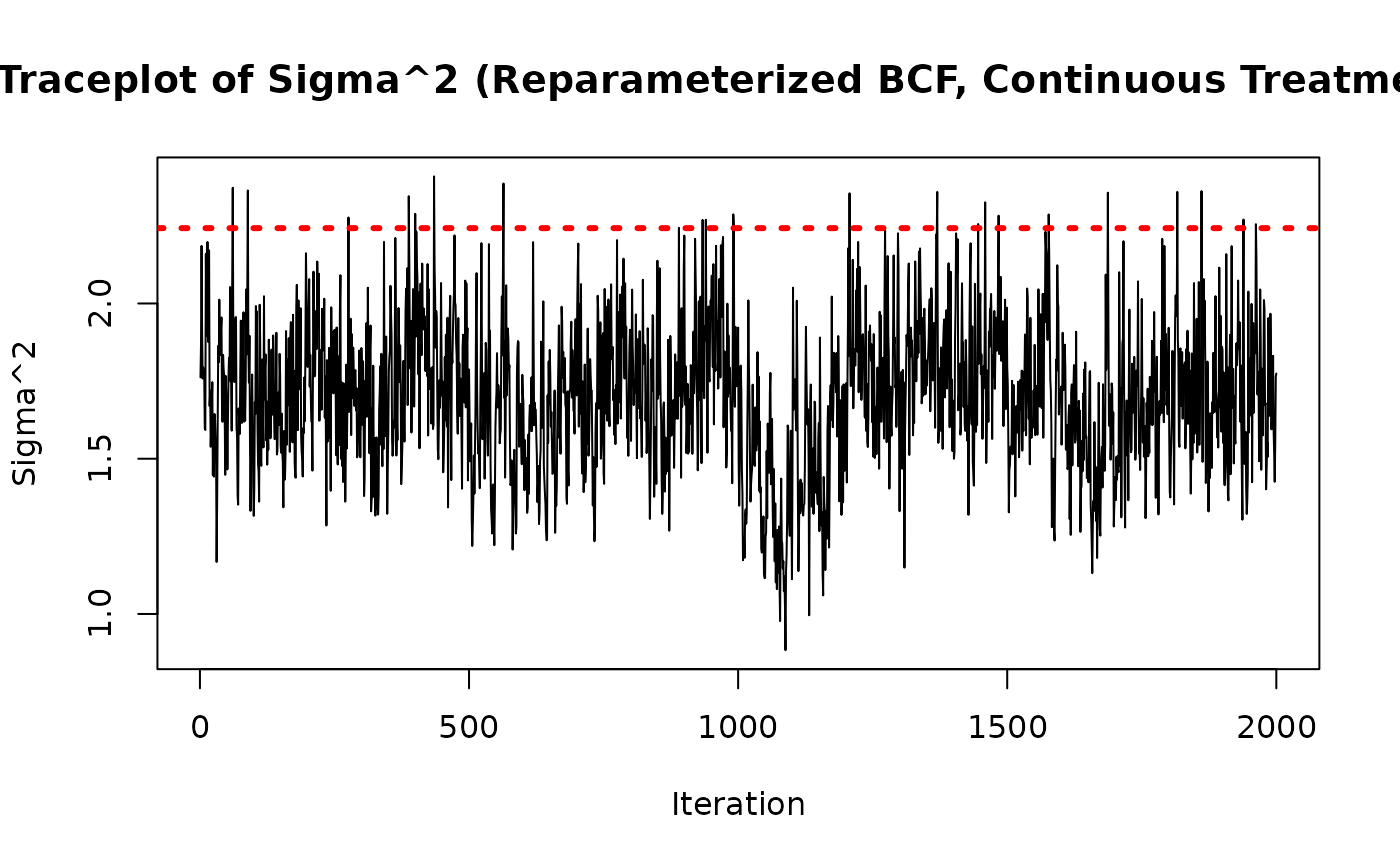

As in the binary treatment case, $\tau_0$ and $\bar{t}(X)$ are negatively correlated across posterior draws

tau_0_posterior <- extractParameter(bcf_model_reparam, "tau_0")
t_x_posterior <- predict(
  bcf_model_reparam,
  X = X_test,
  Z = Z_test,
  propensity = pi_test,
  type = "posterior",
  terms = "tau"
)
t_x_posterior <- colMeans(t_x_posterior)
plot(
  tau_0_posterior,
  t_x_posterior,
  xlab = "tau_0",
  ylab = "t(X)",
  main = "Posterior of tau_0 vs t(X), averaged over X (Continuous Treatment)"
)

References

Hahn, P Richard, Jared S Murray, and Carlos M Carvalho. 2020. “Bayesian Regression Tree Models for Causal Inference: Regularization, Confounding, and Heterogeneous Effects (with Discussion).” Bayesian Analysis 15 (3): 965–1056.