Bayesian Additive Regression Trees for Supervised Learning

This vignette demonstrates how to sample variants of the BART model (Chipman et al. (2010)), using the bart() function in stochtree. The original BART model is

\[ \begin{aligned} y_i \mid X_i = x_i &\sim \mathcal{N}(f(x_i), \sigma^2)\\ \sigma^2 &\sim \text{IG}\left(\frac{\nu}{2}, \frac{\nu \lambda}{2}\right) \end{aligned} \]

where

\[ f(X) = \sum_{s=1}^m g_s(X) \]

and each \(g_s\) refers to a decision tree function which partitions \(X\) into \(k_s\) mutually exclusive regions (\(\mathcal{A}_s = \mathcal{A}_{s,1} \cup \dots \cup \mathcal{A}_{s,k_s}\)) and assigns a scalar parameter \(\mu_{s,j}\) to each region \(\mathcal{A}_{s,j}\)

\[ g_s(x) = \sum_{j = 1}^{k_s} \mu_{s,j} \mathbb{I}\left(x \in \mathcal{A}_{s,j}\right). \]

The partitions \(\mathcal{A}_s\) are defined by a series of logical split rules \(X_i \leq c\) where \(i\) is a variable index and \(c\) is a numeric cutpoint and these partitions are guided by a uniform prior on variables and cutpoints. The prior on partitions is further specified by a probability of splitting a node

\[ P(\text{split node } \eta) = \alpha (1 + \text{depth}_{\eta})^{-\beta} \]

The prior for each leaf node parameter is

\[ \mu_{s,j} \sim \mathcal{N}\left(0, \sigma^2_{\mu}\right) \]

Together, we refer to this conditional mean model as

\[ f(X) \sim \text{BART}(\alpha, \beta, m) \]

This is the “core” of stochtree’s supervised learning interface, though we support many expanded models including

• linear leaf regression (i.e. each leaf node evaluates a linear regression on basis \(W\) rather than return a constant),
• additive random effects,
• forest-based heteroskedasticity,
• binary / ordinal outcome modeling using the probit and complementary log-log (cloglog) links,

and we offer the ability to sample any of the above models using the MCMC or the Grow-From-Root sampler (He and Hahn (2023)).

Setup

To begin, we load the stochtree and other necessary packages.

R

library(stochtree)

Python

import matplotlib.pyplot as plt
import numpy as np
import pandas as pd
from sklearn.model_selection import train_test_split
from stochtree import BARTModel

We set a seed for reproducibility

R

random_seed <- 1234
set.seed(random_seed)

Python

random_seed = 1234
rng = np.random.default_rng(random_seed)

Demo 1: Step Function

Data Generation

We generate data from a simple step function

R

# Generate the data
n <- 500
p_x <- 10
snr <- 3
X <- matrix(runif(n * p_x), ncol = p_x)
f_XW <- (((0 <= X[, 1]) & (0.25 > X[, 1])) *
  (-7.5) +
  ((0.25 <= X[, 1]) & (0.5 > X[, 1])) * (-2.5) +
  ((0.5 <= X[, 1]) & (0.75 > X[, 1])) * (2.5) +
  ((0.75 <= X[, 1]) & (1 > X[, 1])) * (7.5))
noise_sd <- sd(f_XW) / snr
y <- f_XW + rnorm(n, 0, 1) * noise_sd

Python

# Generate the data
n = 500
p_x = 10
snr = 3
X = rng.uniform(0, 1, (n, p_x))
f_XW = (
    ((X[:, 0] >= 0.0) & (X[:, 0] < 0.25)) * (-7.5)
    + ((X[:, 0] >= 0.25) & (X[:, 0] < 0.5)) * (-2.5)
    + ((X[:, 0] >= 0.5) & (X[:, 0] < 0.75)) * (2.5)
    + ((X[:, 0] >= 0.75) & (X[:, 0] < 1.0)) * (7.5)
)
noise_sd = np.std(f_XW) / snr
y = f_XW + rng.normal(0, noise_sd, n)

Split the data into train and test sets

R

test_set_pct <- 0.2
n_test <- round(test_set_pct * n)
n_train <- n - n_test
test_inds <- sort(sample(1:n, n_test, replace = FALSE))
train_inds <- (1:n)[!((1:n) %in% test_inds)]
X_test <- as.data.frame(X[test_inds, ])
X_train <- as.data.frame(X[train_inds, ])
y_test <- y[test_inds]
y_train <- y[train_inds]

Python

test_set_pct = 0.2
X_train, X_test, y_train, y_test = train_test_split(
    X, y, test_size=test_set_pct, random_state=random_seed
)

Sampling and Analysis

We sample from a BART model of \(y \mid X\) with 10 grow-from-root GFR samples (He and Hahn (2023)) followed by 100 MCMC samples (this is the default in stochtree), run for 4 chains initialized by different GFR iterations.

We also specify \(m = 100\) trees and we let both \(\sigma^2\) and \(\sigma^2_{\mu}\) be updated by Gibbs samplers.

R

num_gfr <- 10
num_burnin <- 0
num_mcmc <- 100
general_params <- list(
  sample_sigma2_global = T,
  num_threads = 1,
  num_chains = 4,
  random_seed = random_seed
)
mean_forest_params <- list(sample_sigma2_leaf = T, num_trees = 100)
bart_model <- stochtree::bart(
  X_train = X_train,
  y_train = y_train,
  X_test = X_test,
  num_gfr = num_gfr,
  num_burnin = num_burnin,
  num_mcmc = num_mcmc,
  general_params = general_params,
  mean_forest_params = mean_forest_params
)

Python

num_gfr = 10
num_burnin = 0
num_mcmc = 100
general_params = {
    "sample_sigma2_global": True,
    "num_threads": 1,
    "num_chains": 4,
    "random_seed": random_seed,
}
mean_forest_params = {"sample_sigma2_leaf": True, "num_trees": 100}
bart_model = BARTModel()
bart_model.sample(
    X_train=X_train,
    y_train=y_train,
    X_test=X_test,
    num_gfr=num_gfr,
    num_burnin=num_burnin,
    num_mcmc=num_mcmc,
    general_params=general_params,
    mean_forest_params=mean_forest_params,
)

Plot the mean outcome predictions versus the true outcomes

R

y_hat_test <- predict(
  bart_model,
  X = X_test, 
  terms = "y_hat", 
  type = "mean"
)
plot(
  y_hat_test,
  y_test,
  xlab = "predicted",
  ylab = "actual",
  main = "Outcome"
)
abline(0, 1, col = "red", lty = 3, lwd = 3)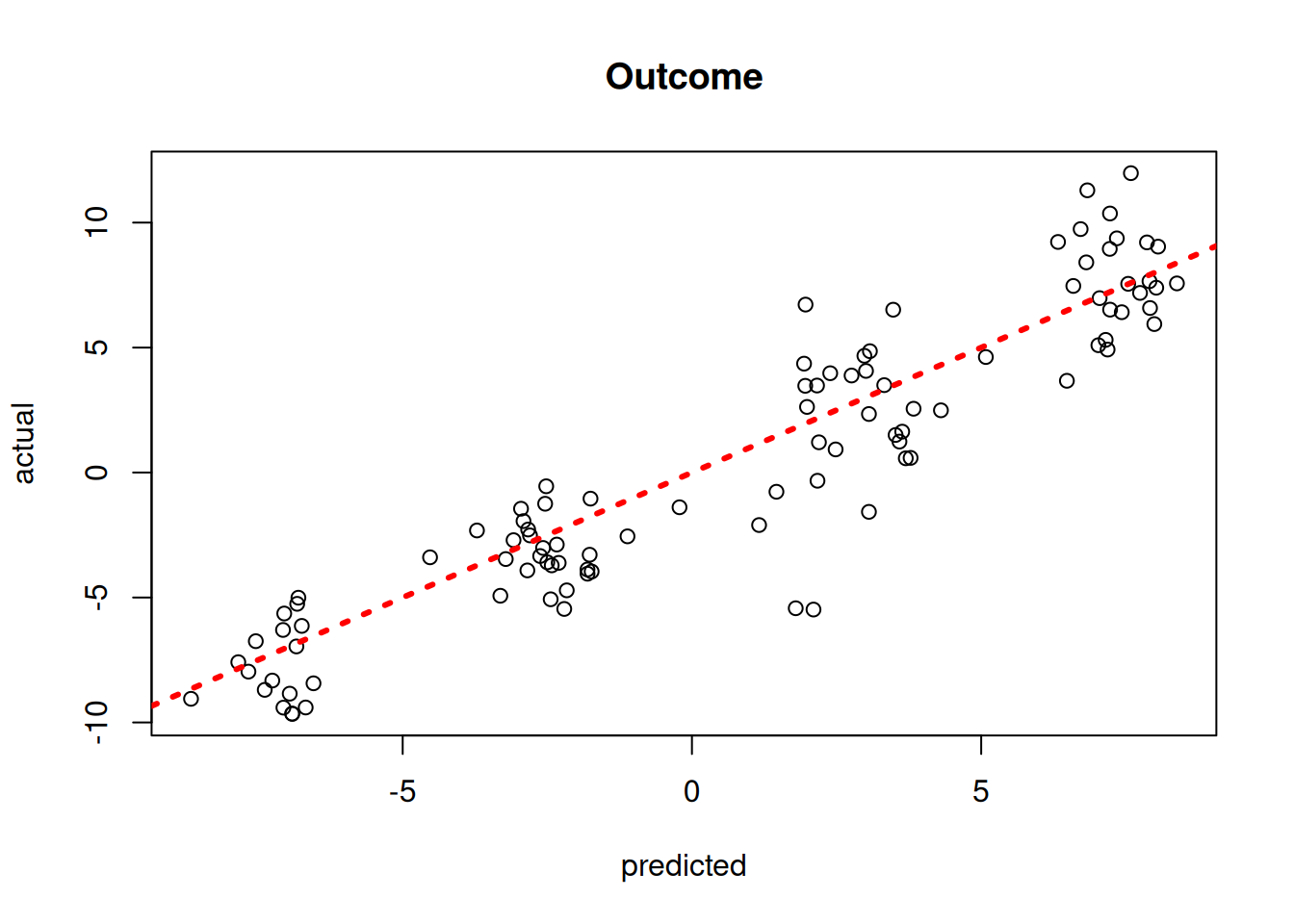

Python

y_hat_test = bart_model.predict(X=X_test, terms="y_hat", type="mean")
lo, hi = min(y_hat_test.min(), y_test.min()), max(y_hat_test.max(), y_test.max())
plt.scatter(y_hat_test, y_test, alpha=0.5)
plt.plot([lo, hi], [lo, hi], color="red", linestyle="dashed", linewidth=2)
plt.xlabel("Predicted")
plt.ylabel("Actual")
plt.title("Outcome")
plt.show()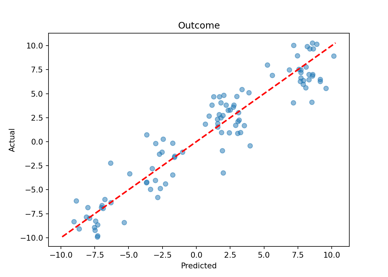

Plot the \(\sigma^2\) traceplot

R

sigma_observed <- var(y - f_XW)
sigma2_global_samples <- extractParameter(bart_model, "sigma2_global")
plot_bounds <- c(
  min(c(sigma2_global_samples, sigma_observed)),
  max(c(sigma2_global_samples, sigma_observed))
)
plot(
  sigma2_global_samples,
  ylim = plot_bounds,
  ylab = "sigma^2",
  xlab = "Sample",
  main = "Global variance parameter"
)
abline(h = sigma_observed, lty = 3, lwd = 3, col = "blue")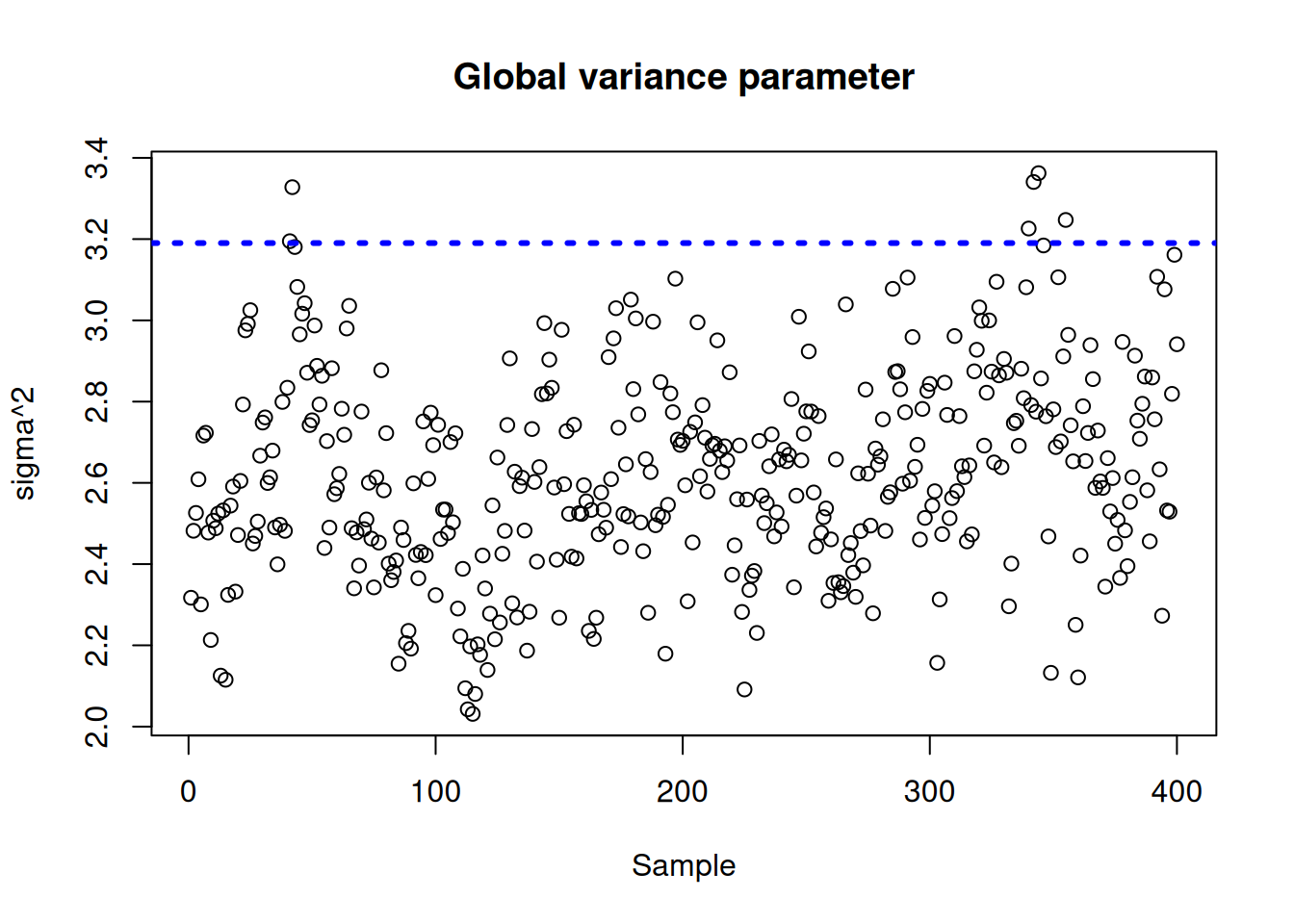

Python

sigma_observed = np.var(y - f_XW)
global_var_samples = bart_model.extract_parameter("sigma2_global")
plt.plot(global_var_samples)
plt.axhline(sigma_observed, color="blue", linestyle="dashed", linewidth=2)
plt.xlabel("Sample")
plt.ylabel(r"$\sigma^2$")
plt.title("Global variance parameter")
plt.show()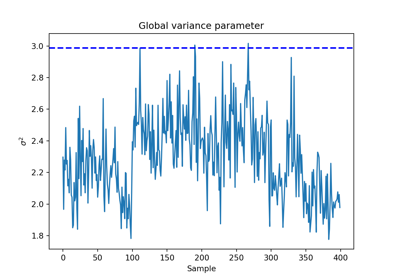

References

Chipman, Hugh A., Edward I. George, and Robert E. McCulloch. 2010. “BART: Bayesian additive regression trees.” The Annals of Applied Statistics 4 (1): 266–98. https://doi.org/10.1214/09-AOAS285.

He, Jingyu, and P Richard Hahn. 2023. “Stochastic Tree Ensembles for Regularized Nonlinear Regression.” Journal of the American Statistical Association 118 (541): 551–70.