BART with a Forest-based Variance Model

This vignette demonstrates how to configure a “variance forest” in stochtree for modeling conditional variance (see Murray (2021)).

Setup

Load necessary packages

R

library(stochtree)

Python

import numpy as np
import matplotlib.pyplot as plt
from stochtree import BARTModel

Set a random seed

R

random_seed = 1234
set.seed(random_seed)

Python

random_seed = 1234
rng = np.random.default_rng(random_seed)

Demo 1: Variance-Only Simulation (Simple DGP)

Here, we generate data with a constant (zero) mean and a relatively simple covariate-modified variance function.

\[\begin{equation*} \begin{aligned} y &= 0 + \sigma(X) \epsilon\\ \sigma^2(X) &= \begin{cases} 0.5 & X_1 \geq 0 \text{ and } X_1 < 0.25\\ 1 & X_1 \geq 0.25 \text{ and } X_1 < 0.5\\ 2 & X_1 \geq 0.5 \text{ and } X_1 < 0.75\\ 3 & X_1 \geq 0.75 \text{ and } X_1 < 1\\ \end{cases}\\ X_1,\dots,X_p &\sim \text{U}\left(0,1\right)\\ \epsilon &\sim \mathcal{N}\left(0,1\right) \end{aligned} \end{equation*}\]

Simulation

Generate data from the DGP above

R

n <- 1000
p_x <- 10
X <- matrix(runif(n * p_x), ncol = p_x)
f_XW <- 0
s_XW <- (((0 <= X[, 1]) & (0.25 > X[, 1])) *
  (0.5) +
  ((0.25 <= X[, 1]) & (0.5 > X[, 1])) * (1) +
  ((0.5 <= X[, 1]) & (0.75 > X[, 1])) * (2) +
  ((0.75 <= X[, 1]) & (1 > X[, 1])) * (3))
y <- f_XW + rnorm(n, 0, 1) * s_XW

Python

n, p_x = 1000, 10
X = rng.uniform(size=(n, p_x))
s_XW = (
    ((X[:, 0] >= 0) & (X[:, 0] < 0.25)) * 0.5
    + ((X[:, 0] >= 0.25) & (X[:, 0] < 0.5)) * 1.0
    + ((X[:, 0] >= 0.5) & (X[:, 0] < 0.75)) * 2.0
    + ((X[:, 0] >= 0.75) & (X[:, 0] < 1.0)) * 3.0
)
y = rng.normal(size=n) * s_XW

Split into train and test sets

R

test_set_pct <- 0.2
n_test <- round(test_set_pct * n)
n_train <- n - n_test
test_inds <- sort(sample(1:n, n_test, replace = FALSE))
train_inds <- (1:n)[!((1:n) %in% test_inds)]
X_test <- as.data.frame(X[test_inds, ])
X_train <- as.data.frame(X[train_inds, ])
y_test <- y[test_inds]
y_train <- y[train_inds]
s_x_test <- s_XW[test_inds]
s_x_train <- s_XW[train_inds]

Python

test_set_pct = 0.2
n_test = round(test_set_pct * n)
test_inds = rng.choice(n, n_test, replace=False)
train_inds = np.setdiff1d(np.arange(n), test_inds)
X_test, X_train = X[test_inds], X[train_inds]
y_test, y_train = y[test_inds], y[train_inds]
s_x_test, s_x_train = s_XW[test_inds], s_XW[train_inds]

Sampling and Analysis

We sample four chains of the \(\sigma^2(X)\) forest using “warm-start” initialization (He and Hahn (2023)).

We use fewer trees for the variance forest than typically used for mean forests, and we disable sampling a global error scale and omit the mean forest by setting num_trees = 0 in its parameter list.

R

num_gfr <- 10
num_burnin <- 0
num_mcmc <- 100
num_trees <- 20
num_samples <- num_gfr + num_burnin + num_mcmc
general_params <- list(
  sample_sigma2_global = F,
  num_chains = 4,
  num_threads = 1,
  random_seed = random_seed
)
mean_forest_params <- list(sample_sigma2_leaf = F, num_trees = 0)
variance_forest_params <- list(num_trees = num_trees)
bart_model <- stochtree::bart(
  X_train = X_train,
  y_train = y_train,
  X_test = X_test,
  num_gfr = num_gfr,
  num_burnin = num_burnin,
  num_mcmc = num_mcmc,
  general_params = general_params,
  mean_forest_params = mean_forest_params,
  variance_forest_params = variance_forest_params
)

Python

num_gfr = 10
num_burnin = 0
num_mcmc = 100
num_trees = 20
bart_model = BARTModel()
bart_model.sample(
    X_train=X_train,
    y_train=y_train,
    X_test=X_test,
    num_gfr=num_gfr,
    num_burnin=num_burnin,
    num_mcmc=num_mcmc,
    general_params={
        "sample_sigma2_global": False,
        "num_threads": 1,
        "num_chains": 4,
        "random_seed": random_seed,
    },
    mean_forest_params={"sample_sigma2_leaf": False, "num_trees": 0},
    variance_forest_params={"num_trees": num_trees},
)

We inspect the model by plotting the true variance function against its forest-based predictions

R

sigma2_x_hat_test <- predict(
  bart_model,
  X = X_test,
  terms = "variance_forest",
  type = "mean"
)
plot(
  sigma2_x_hat_test,
  s_x_test^2,
  pch = 16,
  cex = 0.75,
  xlab = "Predicted",
  ylab = "Actual",
  main = "Variance function"
)
abline(0, 1, col = "red", lty = 2, lwd = 2.5)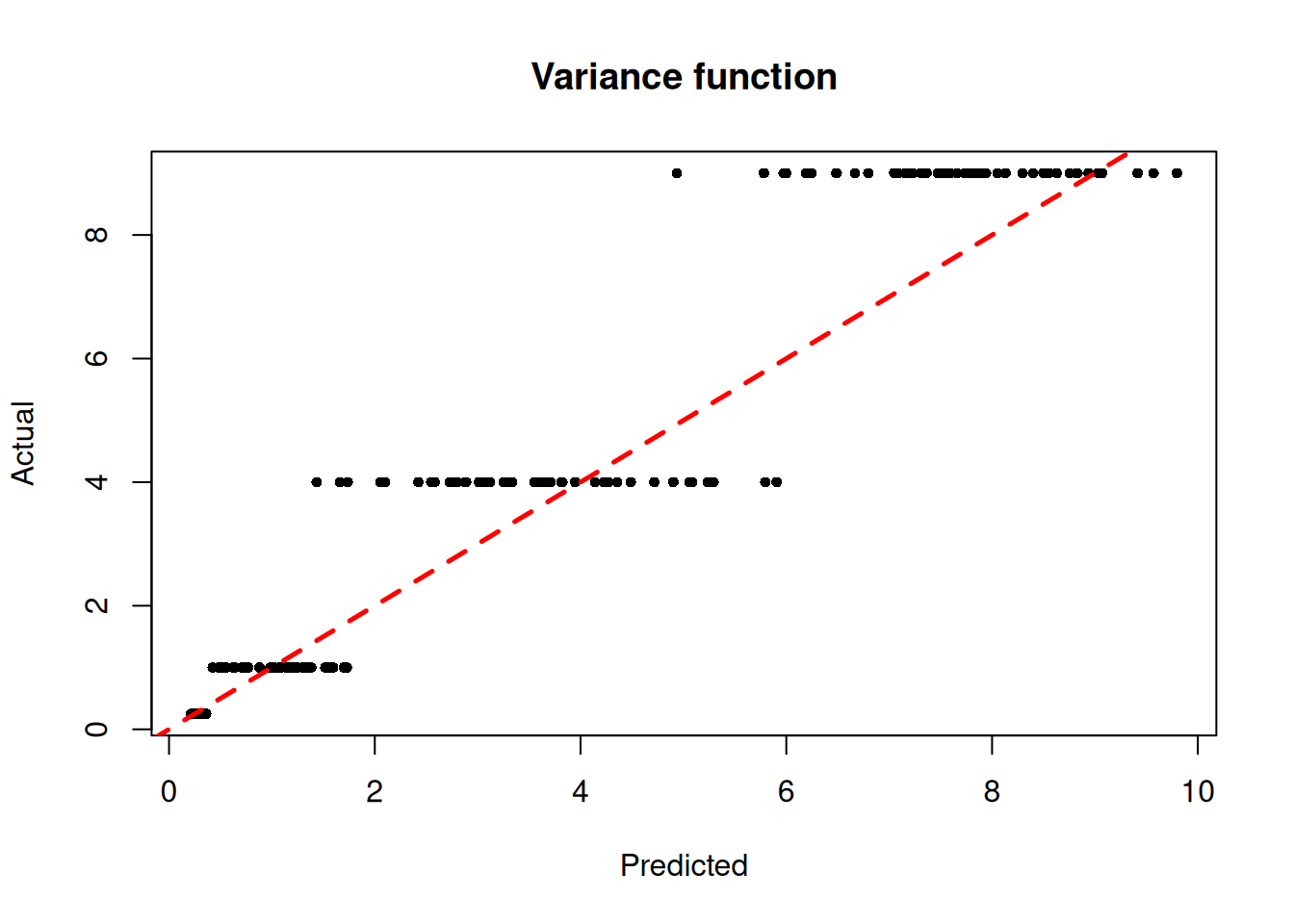

Python

sigma2_x_hat_test = bart_model.predict(X=X_test, terms="variance_forest", type="mean")
lo, hi = (
    min(sigma2_x_hat_test.min(), (s_x_test**2).min()),
    max(sigma2_x_hat_test.max(), (s_x_test**2).max()),
)
plt.scatter(sigma2_x_hat_test, s_x_test**2, s=10, alpha=0.6)
plt.plot([lo, hi], [lo, hi], color="red", linestyle="dashed", linewidth=2)
plt.xlabel("Predicted")
plt.ylabel("Actual")
plt.title("Variance function")
plt.show()

Demo 2: Variance-Only Simulation (Complex DGP)

Here, we generate data with a constant (zero) mean and a more complex covariate-modified variance function.

\[\begin{equation*} \begin{aligned} y &= 0 + \sigma(X) \epsilon\\ \sigma^2(X) &= \begin{cases} 0.25X_3^2 & X_1 \geq 0 \text{ and } X_1 < 0.25\\ 1X_3^2 & X_1 \geq 0.25 \text{ and } X_1 < 0.5\\ 4X_3^2 & X_1 \geq 0.5 \text{ and } X_1 < 0.75\\ 9X_3^2 & X_1 \geq 0.75 \text{ and } X_1 < 1\\ \end{cases}\\ X_1,\dots,X_p &\sim \text{U}\left(0,1\right)\\ \epsilon &\sim \mathcal{N}\left(0,1\right) \end{aligned} \end{equation*}\]

Simulation

We generate data from the DGP above

R

n <- 1000
p_x <- 10
X <- matrix(runif(n*p_x), ncol = p_x)
f_XW <- 0
s_XW <- (
    ((0 <= X[,1]) & (0.25 > X[,1])) * (0.5*X[,3]) +
    ((0.25 <= X[,1]) & (0.5 > X[,1])) * (1*X[,3]) +
    ((0.5 <= X[,1]) & (0.75 > X[,1])) * (2*X[,3]) +
    ((0.75 <= X[,1]) & (1 > X[,1])) * (3*X[,3])
)
y <- f_XW + rnorm(n, 0, 1)*s_XW

Python

n, p_x = 1000, 10
X = rng.uniform(size=(n, p_x))
# R's X[,3] = Python's X[:,2]
s_XW = (
    ((X[:, 0] >= 0)    & (X[:, 0] < 0.25)) * (0.5 * X[:, 2]) +
    ((X[:, 0] >= 0.25) & (X[:, 0] < 0.5))  * (1.0 * X[:, 2]) +
    ((X[:, 0] >= 0.5)  & (X[:, 0] < 0.75)) * (2.0 * X[:, 2]) +
    ((X[:, 0] >= 0.75) & (X[:, 0] < 1.0))  * (3.0 * X[:, 2])
)
y = rng.normal(size=n) * s_XW

And split the data into train and test sets

R

test_set_pct <- 0.2
n_test <- round(test_set_pct*n)
n_train <- n - n_test
test_inds <- sort(sample(1:n, n_test, replace = FALSE))
train_inds <- (1:n)[!((1:n) %in% test_inds)]
X_test <- as.data.frame(X[test_inds,])
X_train <- as.data.frame(X[train_inds,])
y_test <- y[test_inds]
y_train <- y[train_inds]
s_x_test <- s_XW[test_inds]
s_x_train <- s_XW[train_inds]

Python

test_set_pct = 0.2
n_test = round(test_set_pct * n)
test_inds  = rng.choice(n, n_test, replace=False)
train_inds = np.setdiff1d(np.arange(n), test_inds)
X_test,  X_train  = X[test_inds],  X[train_inds]
y_test,  y_train  = y[test_inds],  y[train_inds]
s_x_test, s_x_train = s_XW[test_inds], s_XW[train_inds]

Sampling and Analysis

We sample four chains of the \(\sigma^2(X)\) forest using “warm-start” initialization (He and Hahn (2023)).

We use fewer trees for the variance forest than typically used for mean forests, and we disable sampling a global error scale and omit the mean forest by setting num_trees = 0 in its parameter list.

R

num_gfr <- 10
num_burnin <- 0
num_mcmc <- 100
num_trees <- 20
num_samples <- num_gfr + num_burnin + num_mcmc
general_params <- list(
  sample_sigma2_global = F,
  num_chains = 4,
  num_threads = 1,
  random_seed = random_seed
)
mean_forest_params <- list(sample_sigma2_leaf = F, num_trees = 0)
variance_forest_params <- list(num_trees = num_trees)
bart_model <- stochtree::bart(
  X_train = X_train,
  y_train = y_train,
  X_test = X_test,
  num_gfr = num_gfr,
  num_burnin = num_burnin,
  num_mcmc = num_mcmc,
  general_params = general_params,
  mean_forest_params = mean_forest_params,
  variance_forest_params = variance_forest_params
)

Python

num_gfr = 10
num_burnin = 0
num_mcmc = 100
num_trees = 20
bart_model = BARTModel()
bart_model.sample(
    X_train=X_train,
    y_train=y_train,
    X_test=X_test,
    num_gfr=num_gfr,
    num_burnin=num_burnin,
    num_mcmc=num_mcmc,
    general_params={
        "sample_sigma2_global": False,
        "num_threads": 1,
        "num_chains": 4,
        "random_seed": random_seed,
    },
    mean_forest_params={"sample_sigma2_leaf": False, "num_trees": 0},
    variance_forest_params={"num_trees": num_trees},
)

We inspect the model by plotting the true variance function against its forest-based predictions

R

sigma2_x_hat_test <- predict(
  bart_model,
  X = X_test,
  terms = "variance_forest",
  type = "mean"
)
plot(
  sigma2_x_hat_test,
  s_x_test^2,
  pch = 16,
  cex = 0.75,
  xlab = "Predicted",
  ylab = "Actual",
  main = "Variance function"
)
abline(0, 1, col = "red", lty = 2, lwd = 2.5)

Python

sigma2_x_hat_test = bart_model.predict(X=X_test, terms="variance_forest", type="mean")
lo, hi = (
    min(sigma2_x_hat_test.min(), (s_x_test**2).min()),
    max(sigma2_x_hat_test.max(), (s_x_test**2).max()),
)
plt.scatter(sigma2_x_hat_test, s_x_test**2, s=10, alpha=0.6)
plt.plot([lo, hi], [lo, hi], color="red", linestyle="dashed", linewidth=2)
plt.xlabel("Predicted")
plt.ylabel("Actual")
plt.title("Variance function")
plt.show()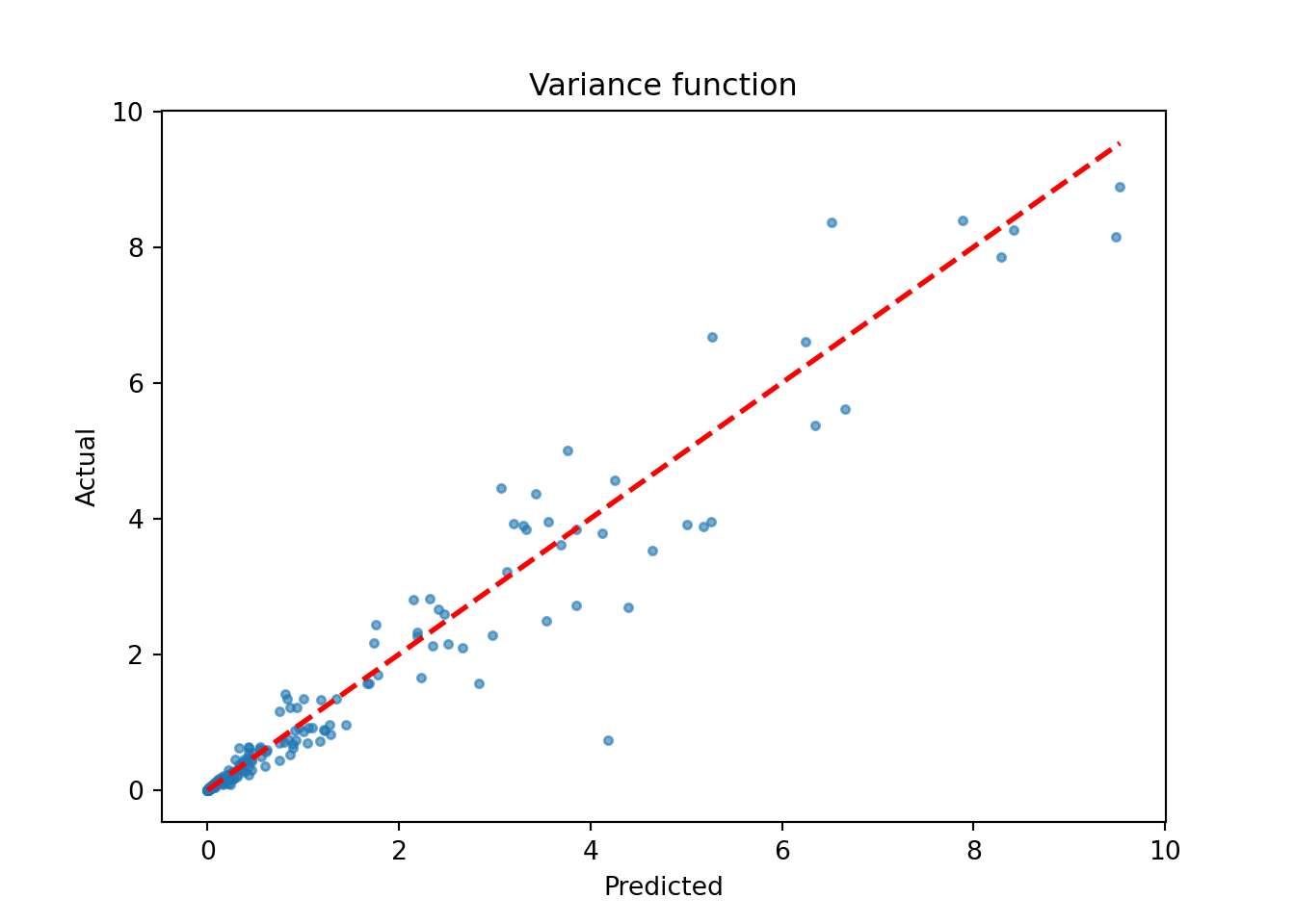

Demo 3: Mean and Variance Function Simulation

Here, we generate data with (relatively simple) covariate-modified mean and variance functions.

\[\begin{equation*} \begin{aligned} y &= f(X) + \sigma(X) \epsilon\\ f(X) &= \begin{cases} -6 & X_2 \geq 0 \text{ and } X_2 < 0.25\\ -2 & X_2 \geq 0.25 \text{ and } X_2 < 0.5\\ 2 & X_2 \geq 0.5 \text{ and } X_2 < 0.75\\ 6 & X_2 \geq 0.75 \text{ and } X_2 < 1\\ \end{cases}\\ \sigma^2(X) &= \begin{cases} 0.25 & X_1 \geq 0 \text{ and } X_1 < 0.25\\ 1 & X_1 \geq 0.25 \text{ and } X_1 < 0.5\\ 4 & X_1 \geq 0.5 \text{ and } X_1 < 0.75\\ 9 & X_1 \geq 0.75 \text{ and } X_1 < 1\\ \end{cases}\\ X_1,\dots,X_p &\sim \text{U}\left(0,1\right)\\ \epsilon &\sim \mathcal{N}\left(0,1\right) \end{aligned} \end{equation*}\]

Simulation

Generate data from the DGP above

R

n <- 1000
p_x <- 10
X <- matrix(runif(n*p_x), ncol = p_x)
f_XW <- (
    ((0 <= X[,2]) & (0.25 > X[,2])) * (-6) +
    ((0.25 <= X[,2]) & (0.5 > X[,2])) * (-2) +
    ((0.5 <= X[,2]) & (0.75 > X[,2])) * (2) +
    ((0.75 <= X[,2]) & (1 > X[,2])) * (6)
)
s_XW <- (
    ((0 <= X[,1]) & (0.25 > X[,1])) * (0.5) +
    ((0.25 <= X[,1]) & (0.5 > X[,1])) * (1) +
    ((0.5 <= X[,1]) & (0.75 > X[,1])) * (2) +
    ((0.75 <= X[,1]) & (1 > X[,1])) * (3)
)
y <- f_XW + rnorm(n, 0, 1)*s_XW

Python

n, p_x = 1000, 10
X = rng.uniform(size=(n, p_x))
f_XW = (
    ((X[:, 1] >= 0)    & (X[:, 1] < 0.25)) * (-6) +
    ((X[:, 1] >= 0.25) & (X[:, 1] < 0.5))  * (-2) +
    ((X[:, 1] >= 0.5)  & (X[:, 1] < 0.75)) * (2)  +
    ((X[:, 1] >= 0.75) & (X[:, 1] < 1.0))  * (6)
)
s_XW = (
    ((X[:, 0] >= 0)    & (X[:, 0] < 0.25)) * 0.5 +
    ((X[:, 0] >= 0.25) & (X[:, 0] < 0.5))  * 1.0 +
    ((X[:, 0] >= 0.5)  & (X[:, 0] < 0.75)) * 2.0 +
    ((X[:, 0] >= 0.75) & (X[:, 0] < 1.0))  * 3.0
)
y = f_XW + rng.normal(size=n) * s_XW

Split the data into train and test sets

R

test_set_pct <- 0.2
n_test <- round(test_set_pct*n)
n_train <- n - n_test
test_inds <- sort(sample(1:n, n_test, replace = FALSE))
train_inds <- (1:n)[!((1:n) %in% test_inds)]
X_test <- as.data.frame(X[test_inds,])
X_train <- as.data.frame(X[train_inds,])
y_test <- y[test_inds]
y_train <- y[train_inds]
f_x_test <- f_XW[test_inds]
s_x_test <- s_XW[test_inds]

Python

test_set_pct = 0.2
n_test = round(test_set_pct * n)
test_inds  = rng.choice(n, n_test, replace=False)
train_inds = np.setdiff1d(np.arange(n), test_inds)
X_test,  X_train  = X[test_inds],  X[train_inds]
y_test,  y_train  = y[test_inds],  y[train_inds]
f_x_test = f_XW[test_inds]
s_x_test = s_XW[test_inds]

Sampling and Analysis

As above, we sample four chains of the \(\sigma^2(X)\) forest using “warm-start” initialization (He and Hahn (2023)), except we do not omit the mean forest by setting num_trees = 0.

R

num_gfr <- 10
num_burnin <- 0
num_mcmc <- 100
general_params <- list(
  sample_sigma2_global = F,
  num_threads = 1,
  num_chains = 4,
  random_seed = random_seed
)
mean_forest_params <- list(
  sample_sigma2_leaf = F,
  num_trees = 50,
  alpha = 0.95,
  beta = 2,
  min_samples_leaf = 5
)
variance_forest_params <- list(
  num_trees = 50,
  alpha = 0.95,
  beta = 1.25,
  min_samples_leaf = 5
)
bart_model <- stochtree::bart(
  X_train = X_train,
  y_train = y_train,
  X_test = X_test,
  num_gfr = num_gfr,
  num_burnin = num_burnin,
  num_mcmc = num_mcmc,
  general_params = general_params,
  mean_forest_params = mean_forest_params,
  variance_forest_params = variance_forest_params
)

Python

bart_model = BARTModel()
bart_model.sample(
    X_train=X_train,
    y_train=y_train,
    X_test=X_test,
    num_gfr=10,
    num_burnin=0,
    num_mcmc=100,
    general_params={
        "sample_sigma2_global": False,
        "num_threads": 1,
        "num_chains": 4,
        "random_seed": random_seed,
    },
    mean_forest_params={
        "sample_sigma2_leaf": False,
        "num_trees": 50,
        "alpha": 0.95,
        "beta": 2,
        "min_samples_leaf": 5,
    },
    variance_forest_params={
        "num_trees": 50,
        "alpha": 0.95,
        "beta": 1.25,
        "min_samples_leaf": 5,
    },
)

We inspect the model by plotting the true variance function against the variance forest predictions

R

sigma2_x_hat_test <- predict(
  bart_model,
  X = X_test,
  terms = "variance_forest",
  type = "mean"
)
plot(
  sigma2_x_hat_test,
  s_x_test^2,
  pch = 16,
  cex = 0.75,
  xlab = "Predicted",
  ylab = "Actual",
  main = "Variance function"
)
abline(0, 1, col = "red", lty = 2, lwd = 2.5)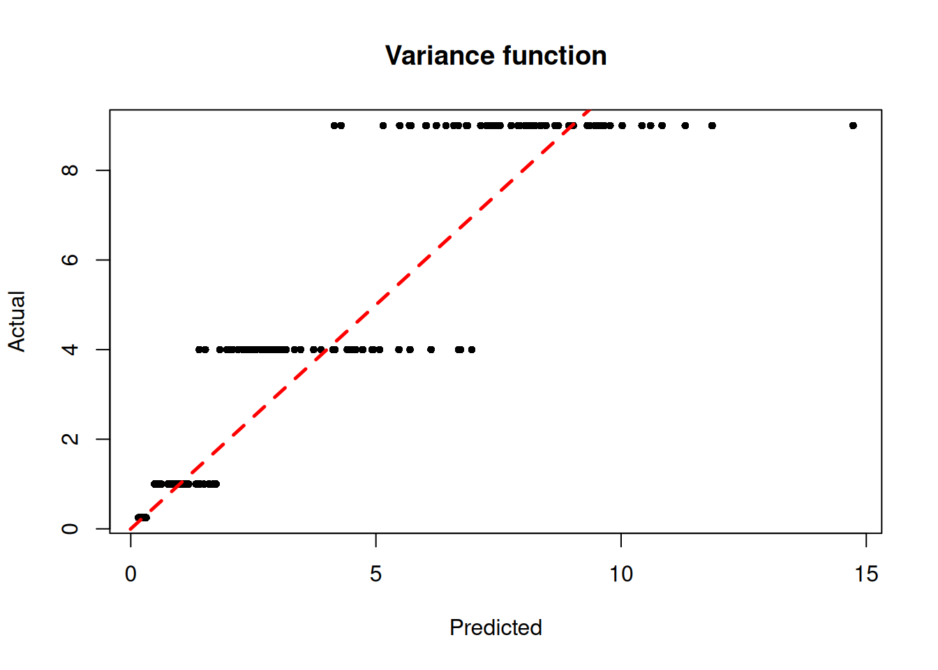

Python

sigma2_x_hat_test = bart_model.predict(X=X_test, terms="variance_forest", type="mean")
lo, hi = (
    min(sigma2_x_hat_test.min(), (s_x_test**2).min()),
    max(sigma2_x_hat_test.max(), (s_x_test**2).max()),
)
plt.scatter(sigma2_x_hat_test, s_x_test**2, s=10, alpha=0.6)
plt.plot([lo, hi], [lo, hi], color="red", linestyle="dashed", linewidth=2)
plt.xlabel("Predicted")
plt.ylabel("Actual")
plt.title("Variance function")
plt.show()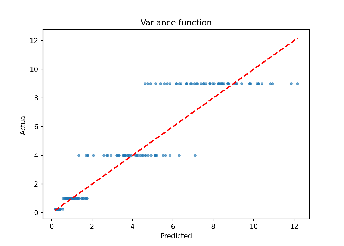

We also plot the true outcome against mean forest predictions

R

y_hat_test <- predict(
  bart_model,
  X = X_test,
  terms = "y_hat",
  type = "mean"
)
plot(
  y_hat_test,
  y_test,
  pch = 16,
  cex = 0.75,
  xlab = "Predicted",
  ylab = "Actual",
  main = "Outcome"
)
abline(0, 1, col = "red", lty = 2, lwd = 2.5)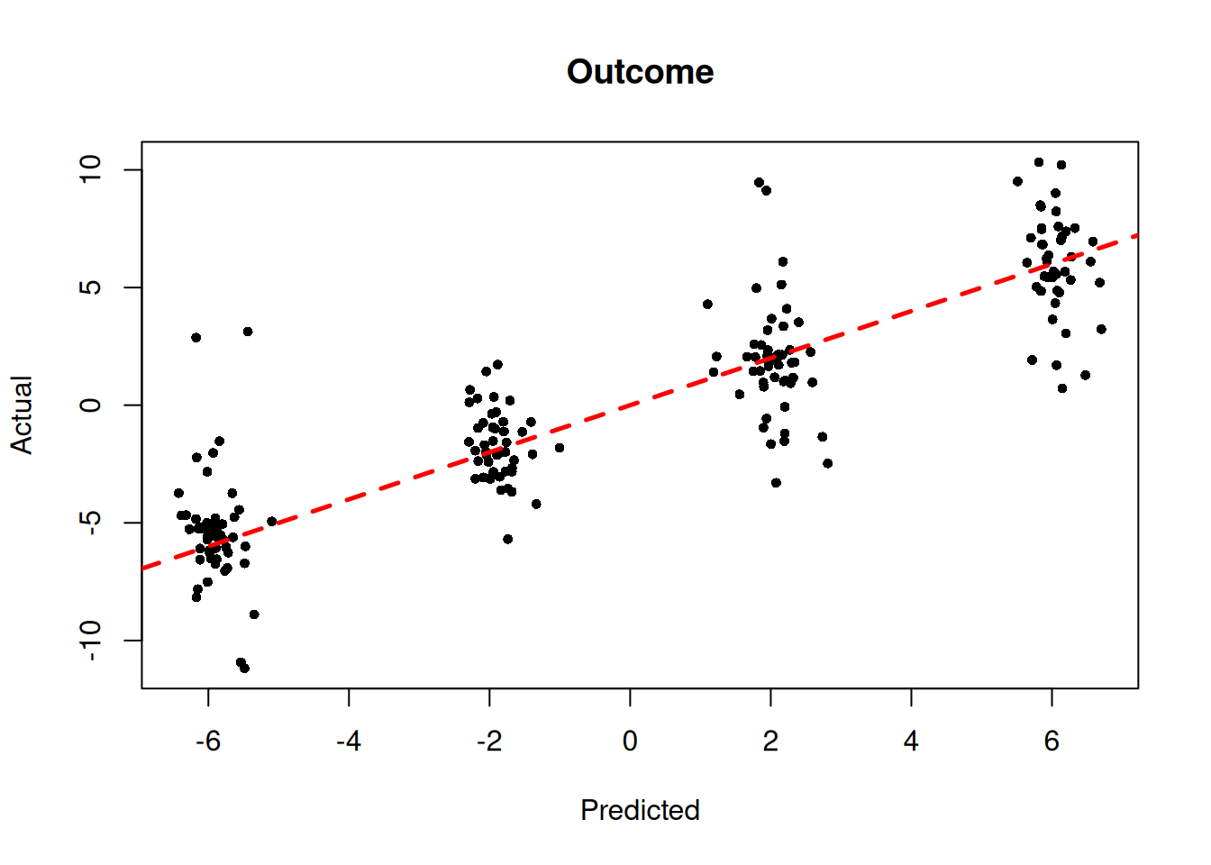

Python

y_hat_test = bart_model.predict(X=X_test, terms="y_hat", type="mean")
lo, hi = (
    min(y_hat_test.min(), y_test.min()),
    max(y_hat_test.max(), y_test.max()),
)
plt.scatter(y_hat_test, y_test, s=10, alpha=0.6)
plt.plot([lo, hi], [lo, hi], color="red", linestyle="dashed", linewidth=2)
plt.xlabel("Predicted")
plt.ylabel("Actual")
plt.title("Outcome")
plt.show()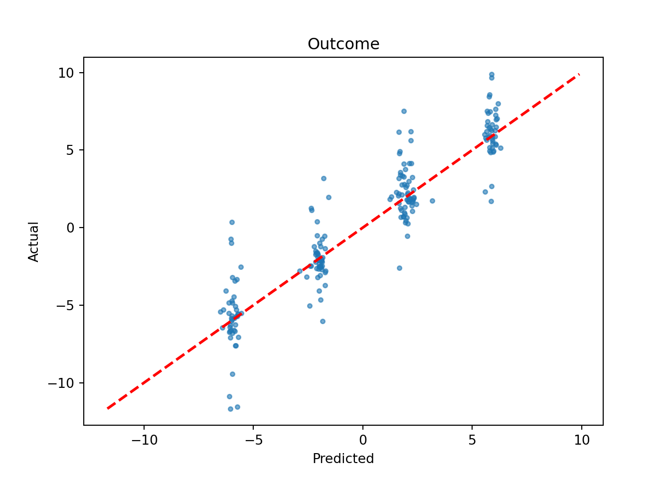

References

He, Jingyu, and P Richard Hahn. 2023. “Stochastic Tree Ensembles for Regularized Nonlinear Regression.” Journal of the American Statistical Association 118 (541): 551–70.

Murray, Jared S. 2021. “Log-Linear Bayesian Additive Regression Trees for Multinomial Logistic and Count Regression Models.” Journal of the American Statistical Association 116 (534): 756–69.