Building a Custom Gibbs Sampler with Stochtree Primitives

While the functions bart() and bcf() provide simple and performant interfaces for supervised learning / causal inference, stochtree also offers access to many of the “low-level” data structures that are typically implemented in C++. This low-level interface is not designed for performance or even simplicity — rather the intent is to provide a “prototype” interface to the C++ code that doesn’t require modifying any C++.

Motivation

To illustrate when such a prototype interface might be useful, consider the classic BART algorithm

Input: \(y\), \(X\), \(\tau\), \(\nu\), \(\lambda\), \(\alpha\), \(\beta\)

Output: \(mc\) samples of a decision forest with \(m\) trees and global variance parameter \(\sigma^2\)

Initialize \(\sigma^2\) via a default or a data-dependent calibration exercise

Initialize a forest with \(m\) trees with a single root node, referring to tree \(j\)’s prediction vector as \(f_{j}\)

Compute residual as \(r = y - \sum_{j=1}^k f_{j}\)

For \(i\) in \(\left\{1,\dots,mc\right\}\):

For \(j\) in \(\left\{1,\dots,m\right\}\):

Add predictions for tree \(j\) to residual: \(r = r + f_{j}\)

Sample tree \(j\) of forest \(i\) from \(p\left(\mathcal{T}_{i,j} \mid r, \sigma^2\right)\)

Sample tree \(j\)’s leaf parameters from \(p\left(\theta_{i,j} \mid \mathcal{T}_{i,j}, r, \sigma^2\right)\) and update \(f_j\) accordingly

Update residual by removing tree \(j\)’s predictions: \(r = r - f_{j}\)

Sample \(\sigma^2\) from \(p\left(\sigma^2 \mid r\right)\)

Return each of the forests and \(\sigma^2\) draws

This algorithm is implemented in stochtree via the bart() R function or the BARTModel python class, but the low-level interface allows you to customize this loop.

In this vignette, we will demonstrate how to use this interface to fit a modified BART model in which the global error variance is modeled as \(t\)-distributed rather than Gaussian.

Setup

R

library(stochtree)

Python

import numpy as np
import matplotlib.pyplot as plt
from stochtree import (
    RNG, Dataset, Forest, ForestContainer, ForestSampler,
    GlobalVarianceModel, LeafVarianceModel, Residual,
    ForestModelConfig, GlobalModelConfig,
)

Set seed for reproducibility

R

random_seed <- 1234
set.seed(random_seed)

Python

random_seed = 1234
rng = np.random.default_rng(random_seed)

Data Generation and Preparation

Consider a modified version of the “Friedman dataset” (Friedman (1991)) with heavy-tailed errors

\[ \begin{aligned} Y_i \mid X_i = x_i &\overset{\text{iid}}{\sim} t_{\nu}\left(f(x_i), \sigma^2\right),\\ f(x) &= 10 \sin \left(\pi x_1 x_2\right) + 20 (x_3 - 1/2)^2 + 10 x_4 + 5 x_5,\\ X_1, \dots, X_p &\overset{\text{iid}}{\sim} \text{U}\left(0,1\right), \end{aligned} \]

where \(t_{\nu}(\mu,\sigma^2)\) represented a generalized \(t\) distribution with location \(\mu\), scale \(\sigma^2\) and \(\nu\) degrees of freedom.

We simulate from this dataset below

R

n <- 1000
p <- 20
X <- matrix(runif(n * p), ncol = p)
m_x <- (10 *
  sin(pi * X[, 1] * X[, 2]) +
  20 * (X[, 3] - 0.5)^2 +
  10 * X[, 4] +
  5 * X[, 5])
sigma2 <- 9
nu <- 2
eps <- rt(n, df = nu) * sqrt(sigma2)
y <- m_x + eps
sigma2_true <- var(eps)

Python

n = 1000
p = 20
X = rng.uniform(low=0.0, high=1.0, size=(n, p))
m_x = (
    10 * np.sin(np.pi * X[:, 0] * X[:, 1])
    + 20 * np.power(X[:, 2] - 0.5, 2.0)
    + 10 * X[:, 3]
    + 5 * X[:, 4]
)
sigma2 = 9
nu = 2
eps = rng.standard_t(df=nu, size=n) * np.sqrt(sigma2)
y = m_x + eps
sigma2_true = np.var(eps)

And we pre-standardize the outcome

R

y_bar <- mean(y)
y_std <- sd(y)
y_standardized <- (y - y_bar) / y_std

Python

y_bar = np.mean(y)
y_std = np.std(y)
y_standardized = (y - y_bar) / y_std

Sampling

We can obtain \(t\)-distributed errors by augmenting the basic BART model with a further prior on the individual variances: \[ \begin{aligned} Y_i \mid (X_i = x_i) &\overset{\text{iid}}{\sim} \mathrm{N}(f(x_i), \phi_i),\\ \phi_i &\overset{\text{iid}}{\sim} \text{IG}\left(\frac{\nu}{2}, \frac{\nu\sigma^2}{2}\right),\\ f &\sim \mathrm{BART}(\alpha,\beta,m). \end{aligned} \] Any Gamma prior on \(\sigma^2\) ensures conditional conjugacy, though for simplicity’s sake we use a log-uniform prior \(\sigma^2\propto 1 / \sigma^2\). In the implementation below, we sample from a “parameter-expanded” variant of this model discussed in Section 12.1 of Gelman et al. (2013), which possesses favorable convergence properties. \[ \begin{aligned} Y_i \mid (X_i = x_i) &\overset{\text{iid}}{\sim} \mathrm{N}(f(x_i), a^2\phi_i),\\ \phi_i &\overset{\text{iid}}{\sim} \text{IG}\left(\frac{\nu}{2}, \frac{\nu\tau^2}{2}\right),\\ a^2 &\propto 1/a^2,\\ \tau^2 &\propto 1/\tau^2,\\ f &\sim \mathrm{BART}(\alpha,\beta,m). \end{aligned} \]

Helper functions

We define several helper functions for Gibbs draws of each of the above parameters.

R

# Sample observation-specific variance parameters phi_i
sample_phi_i <- function(y, dataset, forest, a2, tau2, nu) {
    n <- length(y)
    yhat_forest <- forest$predict(dataset)
    res <- y - yhat_forest
    posterior_shape <- (nu + 1) / 2
    posterior_scale <- (nu * tau2 + (res * res / a2)) / 2
    return(1 / rgamma(n, posterior_shape, rate = posterior_scale))
}

# Sample variance parameter a^2
sample_a2 <- function(y, dataset, forest, phi_i) {
    n <- length(y)
    yhat_forest <- forest$predict(dataset)
    res <- y - yhat_forest
    posterior_shape <- n / 2
    posterior_scale <- (1 / 2) * sum(res * res / phi_i)
    return(1 / rgamma(1, posterior_shape, rate = posterior_scale))
}

# Sample variance parameter tau^2
sample_tau2 <- function(phi_i, nu) {
    n <- length(phi_i)
    posterior_shape <- nu * n / 2
    posterior_scale <- (nu / 2) * sum(1 / phi_i)
    return(1 / rgamma(1, posterior_shape, rate = posterior_scale))
}

Python

def sample_phi_i(
    y: np.array,
    dataset: Dataset,
    forest: Forest,
    a2: float,
    tau2: float,
    nu: float,
    rng: np.random.Generator,
) -> np.array:
    """
    Sample observation-specific variance parameters phi_i
    """
    n = len(y)
    yhat_forest = forest.predict(dataset)
    res = y - yhat_forest
    posterior_shape = (nu + 1) / 2
    posterior_scale = (nu * tau2 + (res * res / a2)) / 2
    return 1 / rng.gamma(shape=posterior_shape, scale=1 / posterior_scale, size=n)


def sample_a2(
    y: np.array,
    dataset: Dataset,
    forest: Forest,
    phi_i: np.array,
    rng: np.random.Generator,
) -> float:
    """
    Sample variance parameter a^2
    """
    n = len(y)
    yhat_forest = forest.predict(dataset)
    res = y - yhat_forest
    posterior_shape = n / 2
    posterior_scale = (1 / 2) * np.sum(res * res / phi_i)
    return 1 / rng.gamma(shape=posterior_shape, scale=1 / posterior_scale, size=1)[0]


def sample_tau2(phi_i: np.array, nu: float, rng: np.random.Generator) -> float:
    """
    Sample variance parameter tau^2
    """
    n = len(phi_i)
    posterior_shape = nu * n / 2
    posterior_scale = (nu / 2) * np.sum(1 / phi_i)
    return 1 / rng.gamma(shape=posterior_shape, scale=1 / posterior_scale, size=1)[0]

Sampling data structures

The underlying C++ codebase centers around a handful of objects and their interactions. We provide R and Python wrappers for these objects to enable greater customization of stochastic tree samplers than can be furnished by the high-level BART and BCF interfaces.

A “Forest Dataset” class manages covariates, bases, and variance weights used in a forest model, and contains methods for updating the underlying data as well as querying numeric attributes of the data (i.e. num_observations, num_covariates, has_basis, etc…). An Outcome / Residual class wraps the model outcome, which is updated in-place during sampling to reflect the full, or partial, residual net of mean forest or random effects predictions. A “Forest Samples” class is a container of sampled tree ensembles, essentially a very thin wrapper around a C++ std::vector of std::unique_ptr to Ensemble objects. A Forest class is a thin wrapper around Ensemble C++ objects, which is used as the “active forest” or “state” of the forest model during sampling. A “Forest Model” class maintains all of the “temporary” data structures used to sample a forest, and its sample_one_iteration() method performs one iteration of the requested forest sampling algorithm (i.e. Metropolis-Hastings or Grow-From-Root). Two different configuration objects (global and forest-specific) manage the parameters needed to run the samplers.

Writing a custom Gibbs sampler with one or more stochastic forest terms requires initializing each of these objects and then deploying them in a sampling loop.

First, we initialize the data objects with covariates and standardized outcomes

R

# Initial values of robust model parameters
tau2_init <- 1.
a2_init <- 1.
sigma2_init <- 1.
phi_i_init <- rep(1., n)

# Initialize data objects
forest_dataset <- createForestDataset(X, variance_weights = 1 / phi_i_init)
outcome <- createOutcome(y_standardized)

Python

# Initial values of robust model parameters
tau2_init = 1.0
a2_init = 1.0
sigma2_init = tau2_init * a2_init
phi_i_init = np.repeat(1.0, n)

# Initialize data objects
forest_dataset = Dataset()
forest_dataset.add_covariates(X)
forest_dataset.add_variance_weights(1.0 / phi_i_init)
residual = Residual(y_standardized)

Next, we initialize random number generator objects, which are essentially wrappers around std::mt19937, which can optionally be seeded for reproducibility.

R

rng <- createCppRNG(random_seed)

Python

cpp_rng = RNG(random_seed)

Next, we initialize the configuration objects. Note that each config has default values so these parameters do not all need to be explicitly set.

R

# Set parameters
outcome_model_type <- 0
leaf_dimension <- 1
num_trees <- 200
feature_types <- as.integer(rep(0, p)) # 0 = numeric
variable_weights <- rep(1 / p, p)

# Initialize config objects
forest_model_config <- createForestModelConfig(
    feature_types = feature_types,
    num_trees = num_trees,
    min_samples_leaf = 5,
    num_features = p,
    num_observations = n,
    variable_weights = variable_weights,
    leaf_dimension = leaf_dimension,
    leaf_model_type = outcome_model_type
)
global_model_config <- createGlobalModelConfig(
    global_error_variance = sigma2_init
)

Python

# Set parameters
outcome_model_type = 0
leaf_dimension = 1
num_trees = 200
feature_types = np.repeat(0, p).astype(int)  # 0 = numeric
var_weights = np.repeat(1 / p, p)

# Initialize config objects
forest_model_config = ForestModelConfig(
    feature_types=feature_types,
    num_trees=num_trees,
    num_features=p,
    num_observations=n,
    variable_weights=var_weights,
    leaf_dimension=leaf_dimension,
    leaf_model_type=outcome_model_type,
)
global_model_config = GlobalModelConfig(global_error_variance=sigma2_init)

Next, we initialize forest model / sampler objects which dispatch the sampling algorithms

R

forest_model <- createForestModel(forest_dataset, forest_model_config, global_model_config)

Python

forest_sampler = ForestSampler(
    forest_dataset, 
    global_model_config, 
    forest_model_config
)

Initialize both the (empty) container of retained forest samples and the “active forest.”

We set the leaf node values for every (single-node) tree in the active forest so that they sum to the mean of the scaled outcome (which is 0 since it was centered).

R

# Create forest container and active forest
forest_samples <- createForestSamples(num_trees, 1, T)
active_forest <- createForest(num_trees, 1, T)

# Initialize the leaves of each tree in the active forest
leaf_init <- mean(y_standardized)
active_forest$prepare_for_sampler(
    forest_dataset,
    outcome,
    forest_model,
    outcome_model_type,
    leaf_init
)

Python

# Create forest container and active forest
forest_container = ForestContainer(num_trees, leaf_dimension, True, False)
active_forest = Forest(num_trees, leaf_dimension, True, False)

# Initialize the leaves of each tree in the active forest
leaf_init = np.mean(y_standardized, keepdims=True)
forest_sampler.prepare_for_sampler(
    forest_dataset,
    residual,
    active_forest,
    outcome_model_type,
    leaf_init,
)

We prepare to run the sampler by initialize empty containers for all of the parametric components of the model (and other intermediate values we track such as RMSE and predicted values).

R

num_burnin <- 3000
num_mcmc <- 1000
sigma2_samples <- rep(NA, num_mcmc)
a2_samples <- rep(NA, num_mcmc)
tau2_samples <- rep(NA, num_mcmc)
phi_i_samples <- matrix(NA, n, num_mcmc)
rmse_samples <- rep(0, num_mcmc)
fhat_samples <- matrix(0, n, num_mcmc)
current_sigma2 <- sigma2_init
current_a2 <- a2_init
current_tau2 <- tau2_init
current_phi_i <- phi_i_init

Python

num_burnin = 3000
num_mcmc = 1000
sigma2_samples = np.empty(num_mcmc)
a2_samples = np.empty(num_mcmc)
tau2_samples = np.empty(num_mcmc)
phi_i_samples = np.empty((n, num_mcmc))
rmse_samples = np.empty(num_mcmc)
fhat_samples = np.empty((n, num_mcmc))
current_sigma2 = sigma2_init
current_a2 = a2_init
current_tau2 = tau2_init
current_phi_i = phi_i_init

Run an MCMC sampler

R

for (i in 1:(num_burnin + num_mcmc)) {
    keep_sample <- i > num_burnin

    # Sample forest
    forest_model$sample_one_iteration(
        forest_dataset,
        outcome,
        forest_samples,
        active_forest,
        rng,
        forest_model_config,
        global_model_config,
        keep_forest = keep_sample,
        gfr = F, 
        num_threads = 1
    )

    # Sample local variance parameters
    current_phi_i <- sample_phi_i(
        y_standardized,
        forest_dataset,
        active_forest,
        current_a2,
        current_tau2,
        nu
    )

    # Sample a2
    current_a2 <- sample_a2(
        y_standardized,
        forest_dataset,
        active_forest,
        current_phi_i
    )
    if (keep_sample) {
        a2_samples[i - num_burnin] <- current_a2 * y_std^2
    }

    # Sample tau2
    current_tau2 <- sample_tau2(current_phi_i, nu)
    if (keep_sample) {
        tau2_samples[i - num_burnin] <- current_tau2 * y_std^2
        sigma2_samples[i - num_burnin] <- current_tau2 * current_a2 * y_std^2
    }

    # Update observation-specific variance weights
    forest_dataset$update_variance_weights(current_phi_i * current_a2)

    # Compute in-sample RMSE and cache mean function samples
    if (keep_sample) {
        yhat_forest <- active_forest$predict(forest_dataset) * y_std + y_bar
        error <- (m_x - yhat_forest)
        rmse_samples[i - num_burnin] <- sqrt(mean(error * error))
        fhat_samples[, i - num_burnin] <- yhat_forest
    }
}

Python

keep_sample = False
for i in range(num_burnin + num_mcmc):
    if i >= num_burnin:
        keep_sample = True

    # Sample from the forest
    forest_sampler.sample_one_iteration(
        forest_container=forest_container,
        forest=active_forest,
        dataset=forest_dataset,
        residual=residual,
        rng=cpp_rng,
        global_config=global_model_config,
        forest_config=forest_model_config,
        keep_forest=keep_sample,
        gfr=False,
        num_threads=1
    )

    # Sample local variance parameters
    current_phi_i = sample_phi_i(
        y_standardized,
        forest_dataset,
        active_forest,
        current_a2,
        current_tau2,
        nu,
        rng,
    )

    # Sample a2
    current_a2 = sample_a2(
        y_standardized,
        forest_dataset,
        active_forest,
        current_phi_i,
        rng,
    )

    # Sample tau2
    current_tau2 = sample_tau2(current_phi_i, nu, rng)
    if keep_sample:
        tau2_samples[i - num_burnin] = current_tau2 * y_std * y_std
        sigma2_samples[i - num_burnin] = current_tau2 * current_a2 * y_std * y_std

    # Update observation-specific variance weights
    forest_dataset.update_variance_weights(current_phi_i * current_a2)

    # Compute in-sample RMSE and cache mean function samples
    if keep_sample:
        yhat_forest = active_forest.predict(forest_dataset) * y_std + y_bar
        error = m_x - yhat_forest
        rmse_samples[i - num_burnin] = np.sqrt(np.mean(error * error))
        fhat_samples[:, i - num_burnin] = yhat_forest

Compute posterior mean of the conditional expectations for the non-robust model

R

m_x_hat_posterior_mean <- rowMeans(fhat_samples)

Python

m_x_hat_posterior_mean = np.mean(fhat_samples, axis=1)

For comparison, we run the same model without robust errors

R

# Initial value of global error variance parameter
sigma2_init <- 1.0

# Initialize data objects
forest_dataset <- createForestDataset(X)
outcome <- createOutcome(y_standardized)

# Random number generator (std::mt19937)
rng <- createCppRNG(random_seed)

# Model configuration
outcome_model_type <- 0
leaf_dimension <- 1
num_trees <- 200
feature_types <- as.integer(rep(0, p)) # 0 = numeric
variable_weights <- rep(1 / p, p)
forest_model_config <- createForestModelConfig(
    feature_types = feature_types,
    num_trees = num_trees,
    num_features = p,
    min_samples_leaf = 5,
    num_observations = n,
    variable_weights = variable_weights,
    leaf_dimension = leaf_dimension,
    leaf_model_type = outcome_model_type
)
global_model_config <- createGlobalModelConfig(
    global_error_variance = sigma2_init
)

# Forest model object
forest_model <- createForestModel(
    forest_dataset,
    forest_model_config,
    global_model_config
)

# "Active forest" (which gets updated by the sample) and
# container of forest samples (which is written to when
# a sample is not discarded due to burn-in / thinning)
forest_samples <- createForestSamples(num_trees, 1, T)
active_forest <- createForest(num_trees, 1, T)

# Initialize the leaves of each tree in the forest
leaf_init <- mean(y_standardized)
active_forest$prepare_for_sampler(
    forest_dataset,
    outcome,
    forest_model,
    outcome_model_type,
    leaf_init
)
active_forest$adjust_residual(forest_dataset, outcome, forest_model, F, F)

# Prepare to run the sampler
global_var_samples <- rep(NA, num_mcmc)
rmse_samples_non_robust <- rep(0, num_mcmc)
fhat_samples_non_robust <- matrix(0, n, num_mcmc)
current_sigma2 <- sigma2_init

# Run the MCMC sampler
for (i in 1:(num_burnin + num_mcmc)) {
    keep_sample <- i > num_burnin

    # Sample forest
    forest_model$sample_one_iteration(
        forest_dataset,
        outcome,
        forest_samples,
        active_forest,
        rng,
        forest_model_config,
        global_model_config,
        keep_forest = keep_sample,
        gfr = F, 
        num_threads = 1
    )

    # Sample global error variance parameter
    current_sigma2 <- sampleGlobalErrorVarianceOneIteration(
        outcome,
        forest_dataset,
        rng,
        1,
        1
    )
    global_model_config$update_global_error_variance(current_sigma2)
    if (keep_sample) {
        global_var_samples[i - num_burnin] <- current_sigma2 * y_std^2
    }

    # Compute in-sample RMSE
    if (keep_sample) {
        yhat_forest <- active_forest$predict(forest_dataset) * y_std + y_bar
        error <- (m_x - yhat_forest)
        rmse_samples_non_robust[i - num_burnin] <- sqrt(mean(error * error))
        fhat_samples_non_robust[, i - num_burnin] <- yhat_forest
    }
}

Python

# Initial value of global error variance parameter
sigma2_init = 1.0

# Initialize data objects
forest_dataset = Dataset()
forest_dataset.add_covariates(X)
residual = Residual(y_standardized)

# Random number generator (std::mt19937)
cpp_rng = RNG(random_seed)

# Model configuration
outcome_model_type = 0
leaf_dimension = 1
num_trees = 200
feature_types = np.repeat(0, p).astype(int)  # 0 = numeric
var_weights = np.repeat(1 / p, p)
global_model_config = GlobalModelConfig(global_error_variance=sigma2_init)
forest_model_config = ForestModelConfig(
    feature_types=feature_types,
    num_trees=num_trees,
    num_features=p,
    num_observations=n,
    variable_weights=var_weights,
    leaf_dimension=leaf_dimension,
    leaf_model_type=outcome_model_type,
)

# Forest model object
forest_sampler = ForestSampler(forest_dataset, global_model_config, forest_model_config)

# "Active forest" (which gets updated by the sample) and
# container of forest samples (which is written to when
# a sample is not discarded due to burn-in / thinning)
active_forest = Forest(num_trees, leaf_dimension, True, False)
forest_container = ForestContainer(num_trees, leaf_dimension, True, False)

# Initialize the leaves of each tree in the mean forest
leaf_init = np.mean(y_standardized, keepdims=True)
forest_sampler.prepare_for_sampler(
    forest_dataset,
    residual,
    active_forest,
    outcome_model_type,
    leaf_init,
)

# Global error variance model
global_var_model = GlobalVarianceModel()

# Prepare to run the sampler
num_burnin = 3000
num_mcmc = 1000
sigma2_samples_non_robust = np.empty(num_mcmc)
rmse_samples_non_robust = np.empty(num_mcmc)
fhat_samples_non_robust = np.empty((n, num_mcmc))
current_sigma2 = sigma2_init

# Run the MCMC sampler
keep_sample = False
for i in range(num_burnin + num_mcmc):
    if i >= num_burnin:
        keep_sample = True

    # Sample from the forest
    forest_sampler.sample_one_iteration(
        forest_container=forest_container,
        forest=active_forest,
        dataset=forest_dataset,
        residual=residual,
        rng=cpp_rng,
        global_config=global_model_config,
        forest_config=forest_model_config,
        keep_forest=keep_sample,
        gfr=False,
        num_threads=1
    )

    # Sample global variance parameter
    current_sigma2 = global_var_model.sample_one_iteration(residual, cpp_rng, 1.0, 1.0)
    global_model_config.update_global_error_variance(current_sigma2)
    if keep_sample:
        sigma2_samples_non_robust[i - num_burnin] = current_sigma2 * y_std * y_std

    # Compute in-sample RMSE and cache mean function samples
    if keep_sample:
        yhat_forest = active_forest.predict(forest_dataset) * y_std + y_bar
        error = m_x - yhat_forest
        rmse_samples_non_robust[i - num_burnin] = np.sqrt(np.mean(error * error))
        fhat_samples_non_robust[:, i - num_burnin] = yhat_forest

Results

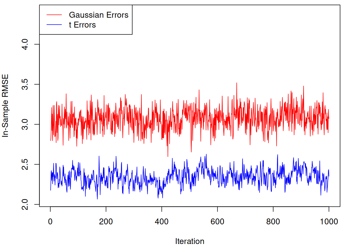
Plot RMSE samples side-by-side

R

par(mar = c(4, 4, 0.5, 0.5))
y_bounds <- range(c(rmse_samples, rmse_samples_non_robust))
y_bounds[2] <- y_bounds[2] * 1.25
plot(
    rmse_samples,
    type = "l",
    col = "blue",
    ylim = y_bounds,
    ylab = "In-Sample RMSE",
    xlab = "Iteration"
)
lines(rmse_samples_non_robust, col = "red")
legend(
    "topleft",
    legend = c("Gaussian Errors", "t Errors"),
    col = c("red", "blue"),
    lty = 1
)

Python

y_bounds = (
    np.min([rmse_samples, rmse_samples_non_robust]) * 0.8,
    np.max([rmse_samples, rmse_samples_non_robust]) * 1.25,
)
plt.ylim(y_bounds)

(1.6380565273939045, 4.317266595742069)

plt.plot(rmse_samples, label="t Errors", color="blue")
plt.plot(
    rmse_samples_non_robust,
    label="Gaussian Errors",
    color="red",
)
plt.ylabel("In-Sample RMSE")
plt.xlabel("Iteration")
plt.legend(loc="upper left")
plt.tight_layout()
plt.show()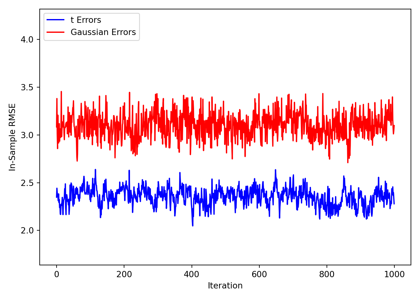

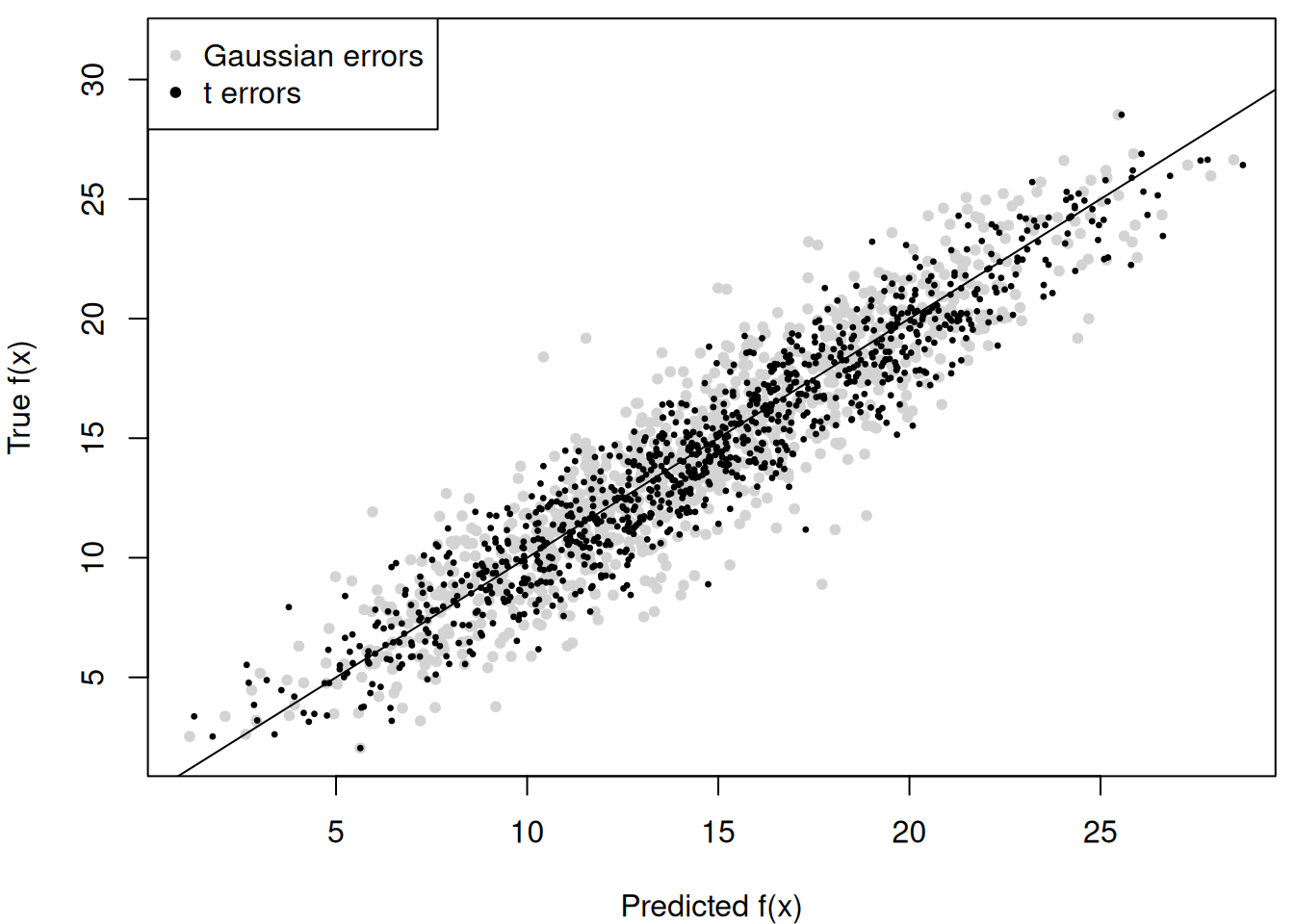
Compute the posterior mean of conditional expectations for the non-robust model and compare to the robust model

R

m_x_hat_posterior_mean_non_robust <- rowMeans(fhat_samples_non_robust)
par(mar = c(4, 4, 0.5, 0.5))
y_bounds <- range(m_x)
y_bounds[2] <- y_bounds[2] * 1.1
plot(
    m_x_hat_posterior_mean_non_robust,
    m_x,
    pch = 20,
    col = 'lightgray',
    xlab = 'Predicted f(x)',
    ylab = 'True f(x)',
    ylim = y_bounds
)
abline(0, 1)
points(m_x_hat_posterior_mean, m_x, pch = 20, cex = 0.5)
legend(
    "topleft",
    legend = c('Gaussian errors', 't errors'),
    pch = c(20, 20),
    col = c('lightgray', 'black')
)

Python

m_x_hat_posterior_mean_non_robust = np.mean(fhat_samples_non_robust, axis=1)
margin = 0.05 * (np.max(m_x) - np.min(m_x))
y_bounds = (np.min(m_x) - margin, np.max(m_x) + margin)
plt.ylim(y_bounds)

(0.008273388343600363, 29.577969135635456)

plt.scatter(
    m_x_hat_posterior_mean_non_robust, m_x, label="Gaussian Errors", color="lightgray"
)
plt.scatter(m_x_hat_posterior_mean, m_x, label="t Errors", color="black")
plt.axline((np.mean(m_x), np.mean(m_x)), slope=1, color="black", linestyle=(0, (3, 3)))
plt.ylabel("True f(x)")
plt.xlabel("Predicted f(x)")
plt.legend(loc="upper left")
plt.tight_layout()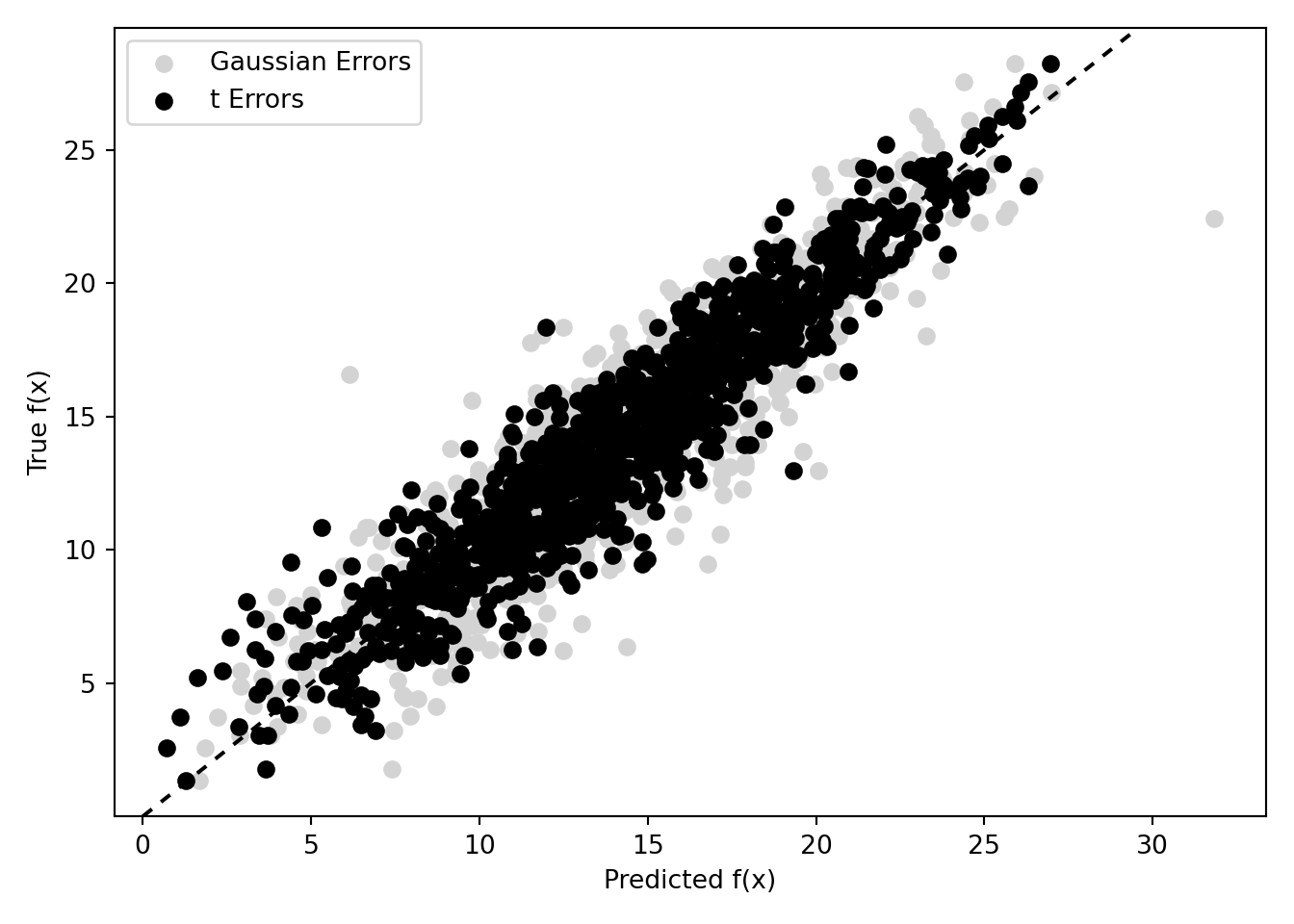

References

Friedman, Jerome H. 1991. “Multivariate Adaptive Regression Splines.” The Annals of Statistics 19 (1): 1–67.

Gelman, Andrew, John B Carlin, Hal S Stern, David B Dunson, Aki Vehtari, and Donald B Rubin. 2013. Bayesian Data Analysis. Third. Chapman; Hall/CRC.