Bayesian Causal Forests for Treatment Effect Estimation

This vignette demonstrates how to use the bcf() function for causal inference (Hahn et al. (2020)). BCF models the conditional average treatment effect (CATE) by fitting two separate tree ensembles

\[ Y_i = \mu(X_i) + \tau(X_i) Z_i + \epsilon_i, \quad \epsilon_i \sim \mathcal{N}(0, \sigma^2) \]

where \(\mu(\cdot)\) is a prognostic forest and \(\tau(\cdot)\) is a treatment effect forest. The estimated propensity score \(\hat{\pi}(X_i)\) is included as a covariate in \(\mu(\cdot)\) to reduce confounding bias.

Setup

Load necessary packages

R

library(stochtree)

Python

import numpy as np
import pandas as pd
import matplotlib.pyplot as plt
from scipy.stats import norm
from stochtree import BCFModel

Set a seed for reproducibility

R

random_seed <- 1234
set.seed(random_seed)

Python

random_seed = 1234
rng = np.random.default_rng(random_seed)

We also define several simple functions that configure the data generating processes used in this vignette

R

g <- function(x) {
  ifelse(x[, 5] == 1, 2, ifelse(x[, 5] == 2, -1, -4))
}
mu1 <- function(x) {
  1 + g(x) + x[, 1] * x[, 3]
}
mu2 <- function(x) {
  1 + g(x) + 6 * abs(x[, 3] - 1)
}
tau1 <- function(x) {
  rep(3, nrow(x))
}
tau2 <- function(x) {
  1 + 2 * x[, 2] * x[, 4]
}

Python

def g(x):
    return np.where(x[:, 4] == 1, 2, np.where(x[:, 4] == 2, -1, -4))


def mu1(x):
    return 1 + g(x) + x[:, 0] * x[:, 2]


def mu2(x):
    return 1 + g(x) + 6 * np.abs(x[:, 2] - 1)


def tau1(x):
    return np.full(x.shape[0], 3.0)


def tau2(x):
    return 1 + 2 * x[:, 1] * x[:, 3]

Binary Treatment

Demo 1: Linear Outcome Model, Heterogeneous Treatment Effect

We consider the following data generating process from Hahn et al. (2020):

\[\begin{equation*} \begin{aligned} y &= \mu(X) + \tau(X) Z + \epsilon\\ \epsilon &\sim N\left(0,\sigma^2\right)\\ \mu(X) &= 1 + g(X) + 6 X_1 X_3\\ \tau(X) &= 1 + 2 X_2 X_4\\ g(X) &= \mathbb{I}(X_5=1) \times 2 - \mathbb{I}(X_5=2) \times 1 - \mathbb{I}(X_5=3) \times 4\\ s_{\mu} &= \sqrt{\mathbb{V}(\mu(X))}\\ \pi(X) &= 0.8 \phi\left(\frac{3\mu(X)}{s_{\mu}}\right) - \frac{X_1}{2} + \frac{2U+1}{20}\\ X_1,X_2,X_3 &\sim N\left(0,1\right)\\ X_4 &\sim \text{Bernoulli}(1/2)\\ X_5 &\sim \text{Categorical}(1/3,1/3,1/3)\\ U &\sim \text{Uniform}\left(0,1\right)\\ Z &\sim \text{Bernoulli}\left(\pi(X)\right) \end{aligned} \end{equation*}\]

Simulation

We generate data from the DGP defined above

R

n <- 1000
snr <- 3
x1 <- rnorm(n)
x2 <- rnorm(n)
x3 <- rnorm(n)
x4 <- as.numeric(rbinom(n, 1, 0.5))
x5 <- as.numeric(sample(1:3, n, replace = TRUE))
X <- cbind(x1, x2, x3, x4, x5)
p <- ncol(X)
mu_x <- mu1(X)
tau_x <- tau2(X)
pi_x <- 0.8 * pnorm((3 * mu_x / sd(mu_x)) - 0.5 * X[, 1]) + 0.05 + runif(n) / 10
Z <- rbinom(n, 1, pi_x)
E_XZ <- mu_x + Z * tau_x
y <- E_XZ + rnorm(n, 0, 1) * (sd(E_XZ) / snr)
X <- as.data.frame(X)
X$x4 <- factor(X$x4, ordered = TRUE)
X$x5 <- factor(X$x5, ordered = TRUE)

Python

n = 1000
snr = 3
x1 = rng.normal(size=n)
x2 = rng.normal(size=n)
x3 = rng.normal(size=n)
x4 = rng.binomial(1, 0.5, n).astype(float)
x5 = rng.choice([1, 2, 3], size=n).astype(float)
X = np.column_stack([x1, x2, x3, x4, x5])
mu_x = mu1(X)
tau_x = tau2(X)
pi_x = (
    0.8 * norm.cdf((3 * mu_x / np.std(mu_x)) - 0.5 * X[:, 0])
    + 0.05
    + rng.uniform(size=n) / 10
)
Z = rng.binomial(1, pi_x, n).astype(float)
E_XZ = mu_x + Z * tau_x
y = E_XZ + rng.normal(size=n) * (np.std(E_XZ) / snr)
X_df = pd.DataFrame({"x1": x1, "x2": x2, "x3": x3, "x4": x4, "x5": x5})
X_df["x4"] = pd.Categorical(X_df["x4"].astype(int), categories=[0, 1], ordered=True)
X_df["x5"] = pd.Categorical(X_df["x5"].astype(int), categories=[1, 2, 3], ordered=True)

Split data into test and train sets

R

test_set_pct <- 0.2
n_test <- round(test_set_pct * n)
n_train <- n - n_test
test_inds <- sort(sample(1:n, n_test, replace = FALSE))
train_inds <- (1:n)[!((1:n) %in% test_inds)]
X_test <- X[test_inds, ]
X_train <- X[train_inds, ]
pi_test <- pi_x[test_inds]
pi_train <- pi_x[train_inds]
Z_test <- Z[test_inds]
Z_train <- Z[train_inds]
y_test <- y[test_inds]
y_train <- y[train_inds]
mu_test <- mu_x[test_inds]
mu_train <- mu_x[train_inds]
tau_test <- tau_x[test_inds]
tau_train <- tau_x[train_inds]

Python

test_set_pct = 0.2
n_test = round(test_set_pct * n)
n_train = n - n_test
test_inds = rng.choice(n, n_test, replace=False)
train_inds = np.setdiff1d(np.arange(n), test_inds)
X_test = X_df.iloc[test_inds]
X_train = X_df.iloc[train_inds]
pi_test, pi_train = pi_x[test_inds], pi_x[train_inds]
Z_test, Z_train = Z[test_inds], Z[train_inds]
y_test, y_train = y[test_inds], y[train_inds]
mu_test, mu_train = mu_x[test_inds], mu_x[train_inds]
tau_test, tau_train = tau_x[test_inds], tau_x[train_inds]

Sampling and Analysis

We simulate from a BCF model initialized by “warm-start” samples fit with the grow-from-root algorithm (He and Hahn (2023), Krantsevich et al. (2023)). This is the default in stochtree.

R

general_params <- list(
  num_threads=1, 
  num_chains=4, 
  random_seed=random_seed
)
bcf_model <- bcf(
  X_train = X_train,
  Z_train = Z_train,
  y_train = y_train,
  propensity_train = pi_train,
  X_test = X_test,
  Z_test = Z_test,
  num_gfr = 10, 
  num_burnin = 1000, 
  num_mcmc = 100,
  propensity_test = pi_test,
  general_params = general_params
)

Python

general_params = {"num_threads": 1, "num_chains": 4, "random_seed": random_seed}
bcf_model = BCFModel()
bcf_model.sample(
    X_train=X_train,
    Z_train=Z_train,
    y_train=y_train,
    propensity_train=pi_train,
    X_test=X_test,
    Z_test=Z_test,
    num_gfr=10,
    num_burnin=1000,
    num_mcmc=100,
    propensity_test=pi_test,
    general_params=general_params,
)

Plot the true versus estimated prognostic function

R

mu_hat_test <- predict(
  bcf_model,
  X = X_test,
  Z = Z_test,
  propensity = pi_test,
  terms = "prognostic_function"
)
plot(
  rowMeans(mu_hat_test),
  mu_test,
  xlab = "predicted",
  ylab = "actual",
  main = "Prognostic function"
)
abline(0, 1, col = "red", lty = 3, lwd = 3)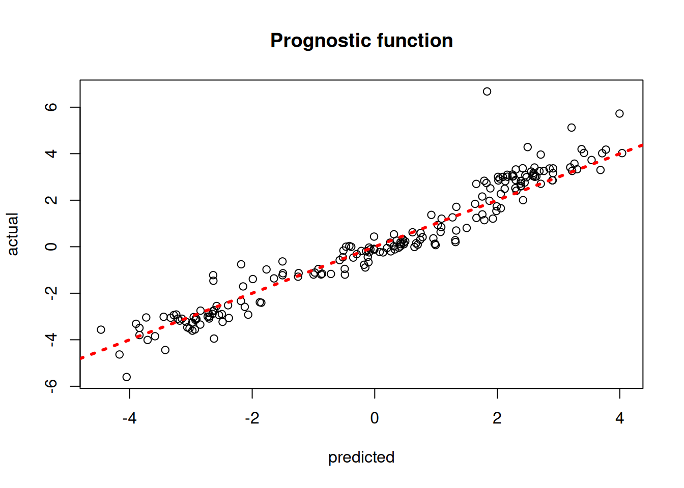

Python

mu_hat_test = bcf_model.predict(
    X=X_test, Z=Z_test, propensity=pi_test, terms="prognostic_function"
)
mu_pred = mu_hat_test.mean(axis=1)
lo, hi = min(mu_pred.min(), mu_test.min()), max(mu_pred.max(), mu_test.max())
plt.scatter(mu_pred, mu_test, alpha=0.5)
plt.plot([lo, hi], [lo, hi], color="red", linestyle="dashed", linewidth=2)
plt.xlabel("Predicted")
plt.ylabel("Actual")
plt.title("Prognostic function")
plt.show()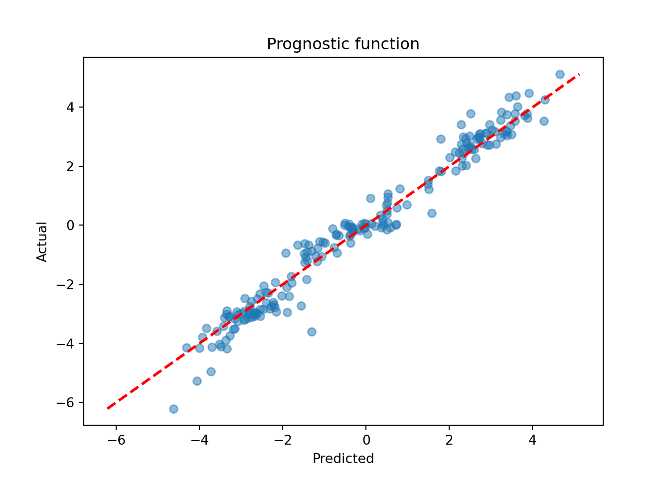

Plot the true versus estimated CATE function

R

tau_hat_test <- predict(
  bcf_model,
  X = X_test,
  Z = Z_test,
  propensity = pi_test,
  terms = "cate"
)
plot(
  rowMeans(tau_hat_test),
  tau_test,
  xlab = "predicted",
  ylab = "actual",
  main = "Treatment effect"
)
abline(0, 1, col = "red", lty = 3, lwd = 3)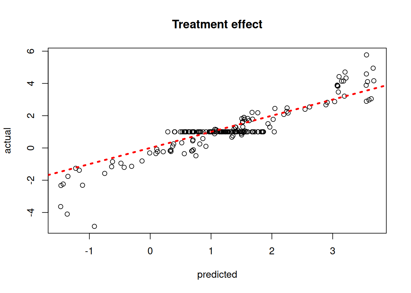

Python

tau_hat_test = bcf_model.predict(X=X_test, Z=Z_test, propensity=pi_test, terms="cate")
tau_pred = tau_hat_test.mean(axis=1)
lo, hi = min(tau_pred.min(), tau_test.min()), max(tau_pred.max(), tau_test.max())
plt.scatter(tau_pred, tau_test, alpha=0.5)
plt.plot([lo, hi], [lo, hi], color="red", linestyle="dashed", linewidth=2)
plt.xlabel("Predicted")
plt.ylabel("Actual")
plt.title("Treatment effect")
plt.show()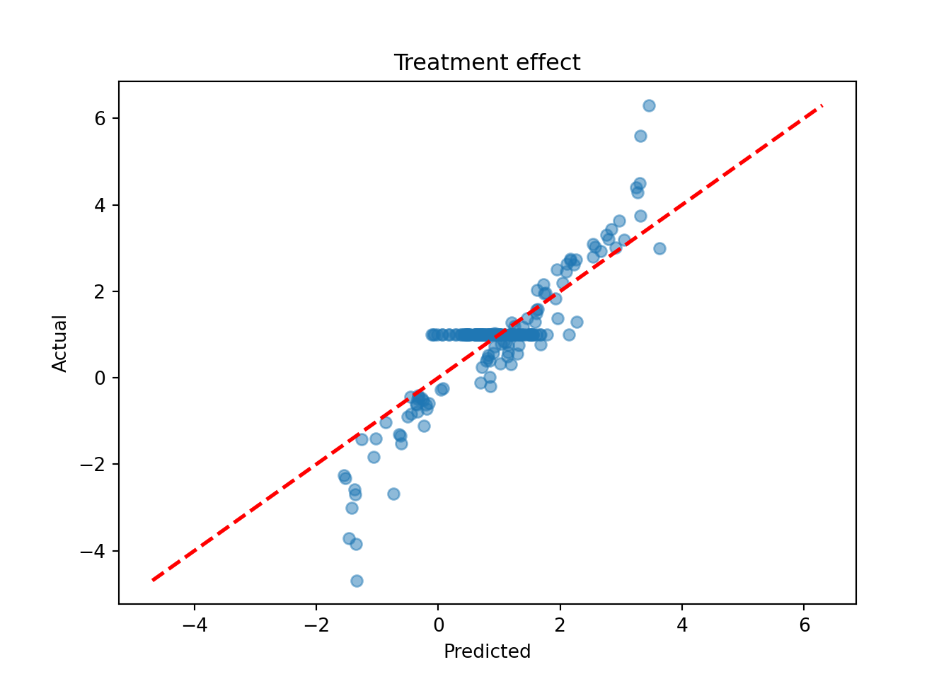

Plot the \(\sigma^2\) traceplot

R

sigma_observed <- var(y - E_XZ)
sigma2_global_samples <- extractParameter(bcf_model, "sigma2_global")
plot_bounds <- c(
  min(c(sigma2_global_samples, sigma_observed)),
  max(c(sigma2_global_samples, sigma_observed))
)
plot(
  sigma2_global_samples,
  ylim = plot_bounds,
  ylab = "sigma^2",
  xlab = "Sample",
  main = "Global variance parameter"
)
abline(h = sigma_observed, lty = 3, lwd = 3, col = "blue")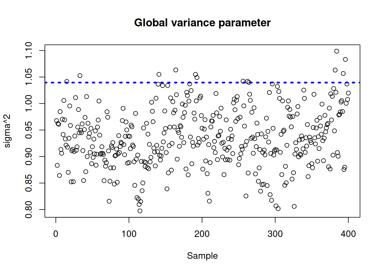

Python

sigma_observed = np.var(y - E_XZ)
global_var_samples = bcf_model.extract_parameter("sigma2_global")
plt.plot(global_var_samples)
plt.axhline(sigma_observed, color="blue", linestyle="dashed", linewidth=2)
plt.xlabel("Sample")
plt.ylabel(r"$\sigma^2$")
plt.title("Global variance parameter")
plt.show()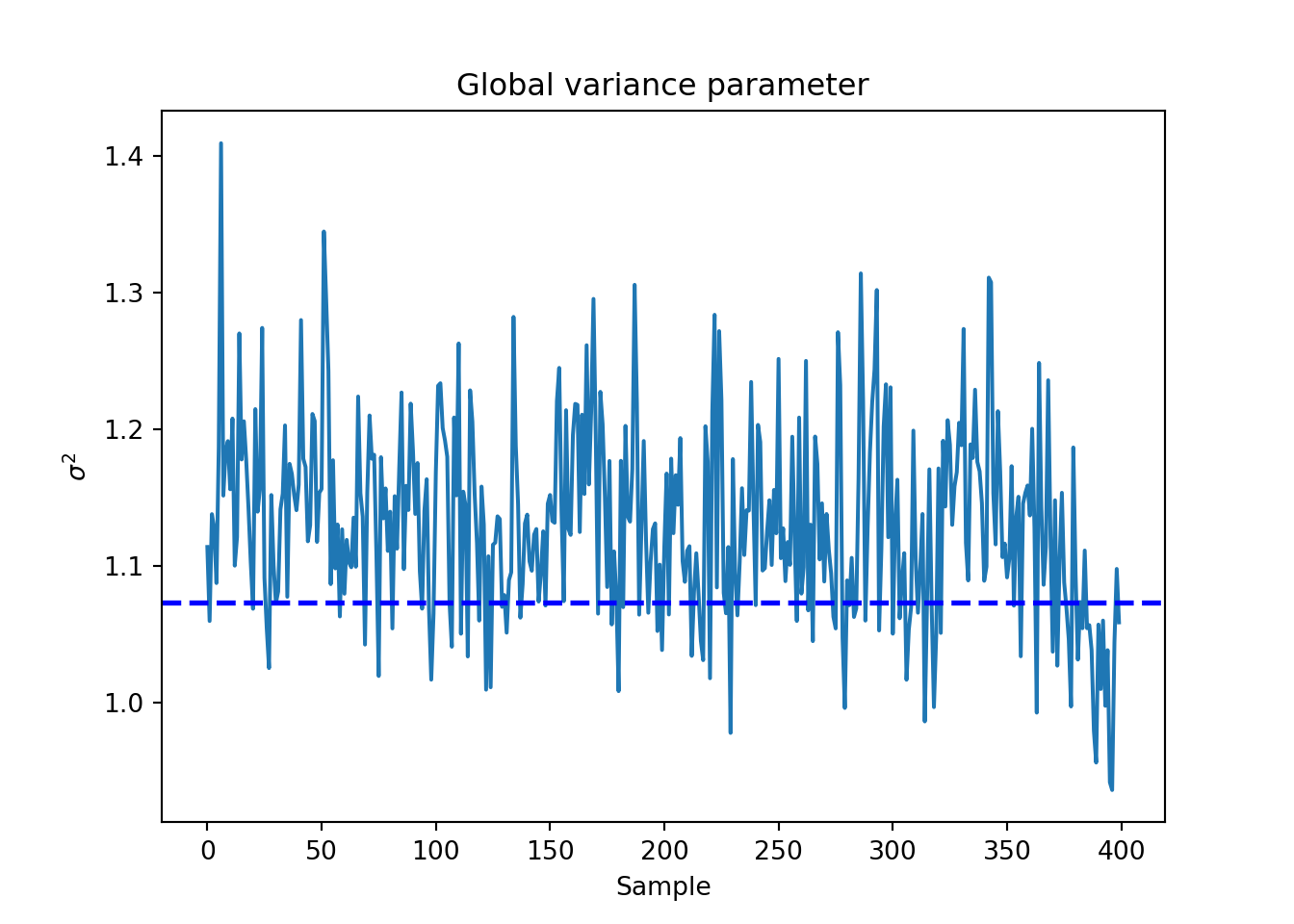

Examine test set interval coverage of \(\tau(X)\).

R

test_lb <- apply(tau_hat_test, 1, quantile, 0.025)
test_ub <- apply(tau_hat_test, 1, quantile, 0.975)
cover <- ((test_lb <= tau_x[test_inds]) &
  (test_ub >= tau_x[test_inds]))
cat("CATE function interval coverage: ", mean(cover) * 100, "%\n")

CATE function interval coverage:  84.5 %

Python

test_lb = np.quantile(tau_hat_test, 0.025, axis=1)
test_ub = np.quantile(tau_hat_test, 0.975, axis=1)
cover = (test_lb <= tau_test) & (test_ub >= tau_test)
print(f"CATE function interval coverage: {cover.mean() * 100:.2f}%")

CATE function interval coverage: 87.50%

Demo 2: Nonlinear Outcome Model, Heterogeneous Treatment Effect

We consider the following data generating process from Hahn et al. (2020):

\[\begin{equation*} \begin{aligned} y &= \mu(X) + \tau(X) Z + \epsilon\\ \epsilon &\sim N\left(0,\sigma^2\right)\\ \mu(X) &= 1 + g(X) + 6 \lvert X_3 - 1 \rvert\\ \tau(X) &= 1 + 2 X_2 X_4\\ g(X) &= \mathbb{I}(X_5=1) \times 2 - \mathbb{I}(X_5=2) \times 1 - \mathbb{I}(X_5=3) \times 4\\ s_{\mu} &= \sqrt{\mathbb{V}(\mu(X))}\\ \pi(X) &= 0.8 \phi\left(\frac{3\mu(X)}{s_{\mu}}\right) - \frac{X_1}{2} + \frac{2U+1}{20}\\ X_1,X_2,X_3 &\sim N\left(0,1\right)\\ X_4 &\sim \text{Bernoulli}(1/2)\\ X_5 &\sim \text{Categorical}(1/3,1/3,1/3)\\ U &\sim \text{Uniform}\left(0,1\right)\\ Z &\sim \text{Bernoulli}\left(\pi(X)\right) \end{aligned} \end{equation*}\]

Simulation

Generate data from the DGP above

R

n <- 1000
snr <- 3
x1 <- rnorm(n)
x2 <- rnorm(n)
x3 <- rnorm(n)
x4 <- as.numeric(rbinom(n, 1, 0.5))
x5 <- as.numeric(sample(1:3, n, replace = TRUE))
X <- cbind(x1, x2, x3, x4, x5)
p <- ncol(X)
mu_x <- mu2(X)
tau_x <- tau2(X)
pi_x <- 0.8 * pnorm((3 * mu_x / sd(mu_x)) - 0.5 * X[, 1]) + 0.05 + runif(n) / 10
Z <- rbinom(n, 1, pi_x)
E_XZ <- mu_x + Z * tau_x
y <- E_XZ + rnorm(n, 0, 1) * (sd(E_XZ) / snr)
X <- as.data.frame(X)
X$x4 <- factor(X$x4, ordered = TRUE)
X$x5 <- factor(X$x5, ordered = TRUE)

Python

n = 1000
snr = 3
x1 = rng.normal(size=n)
x2 = rng.normal(size=n)
x3 = rng.normal(size=n)
x4 = rng.binomial(1, 0.5, n).astype(float)
x5 = rng.choice([1, 2, 3], size=n).astype(float)
X = np.column_stack([x1, x2, x3, x4, x5])
mu_x = mu2(X)  # mu2 for Demo 2
tau_x = tau2(X)
pi_x = (
    0.8 * norm.cdf((3 * mu_x / np.std(mu_x)) - 0.5 * X[:, 0])
    + 0.05
    + rng.uniform(size=n) / 10
)
Z = rng.binomial(1, pi_x, n).astype(float)
E_XZ = mu_x + Z * tau_x
y = E_XZ + rng.normal(size=n) * (np.std(E_XZ) / snr)
X_df = pd.DataFrame({"x1": x1, "x2": x2, "x3": x3, "x4": x4, "x5": x5})
X_df["x4"] = pd.Categorical(X_df["x4"].astype(int), categories=[0, 1], ordered=True)
X_df["x5"] = pd.Categorical(X_df["x5"].astype(int), categories=[1, 2, 3], ordered=True)

Split into train and test sets

R

test_set_pct <- 0.2
n_test <- round(test_set_pct * n)
n_train <- n - n_test
test_inds <- sort(sample(1:n, n_test, replace = FALSE))
train_inds <- (1:n)[!((1:n) %in% test_inds)]
X_test <- X[test_inds, ]
X_train <- X[train_inds, ]
pi_test <- pi_x[test_inds]
pi_train <- pi_x[train_inds]
Z_test <- Z[test_inds]
Z_train <- Z[train_inds]
y_test <- y[test_inds]
y_train <- y[train_inds]
mu_test <- mu_x[test_inds]
mu_train <- mu_x[train_inds]
tau_test <- tau_x[test_inds]
tau_train <- tau_x[train_inds]

Python

test_set_pct = 0.2
n_test = round(test_set_pct * n)
n_train = n - n_test
test_inds = rng.choice(n, n_test, replace=False)
train_inds = np.setdiff1d(np.arange(n), test_inds)
X_test = X_df.iloc[test_inds]
X_train = X_df.iloc[train_inds]
pi_test, pi_train = pi_x[test_inds], pi_x[train_inds]
Z_test, Z_train = Z[test_inds], Z[train_inds]
y_test, y_train = y[test_inds], y[train_inds]
mu_test, mu_train = mu_x[test_inds], mu_x[train_inds]
tau_test, tau_train = tau_x[test_inds], tau_x[train_inds]

Sampling and Analysis

We simulate from a BCF model using default settings.

R

general_params <- list(
  num_threads = 1,
  num_chains = 4,
  random_seed = random_seed
)
bcf_model <- bcf(
  X_train = X_train,
  Z_train = Z_train,
  y_train = y_train,
  propensity_train = pi_train,
  X_test = X_test,
  Z_test = Z_test,
  propensity_test = pi_test,
  num_gfr = 10,
  num_burnin = 1000,
  num_mcmc = 100,
  general_params = general_params
)

Python

general_params = {"num_threads": 1, "num_chains": 4, "random_seed": random_seed}
bcf_model = BCFModel()
bcf_model.sample(
    X_train=X_train,
    Z_train=Z_train,
    y_train=y_train,
    propensity_train=pi_train,
    X_test=X_test,
    Z_test=Z_test,
    propensity_test=pi_test,
    num_gfr=10,
    num_burnin=1000,
    num_mcmc=100,
    general_params=general_params,
)

Plot the true versus estimated prognostic function

R

mu_hat_test <- predict(
  bcf_model,
  X = X_test,
  Z = Z_test,
  propensity = pi_test,
  terms = "prognostic_function"
)
plot(
  rowMeans(mu_hat_test),
  mu_test,
  xlab = "predicted",
  ylab = "actual",
  main = "Prognostic function"
)
abline(0, 1, col = "red", lty = 3, lwd = 3)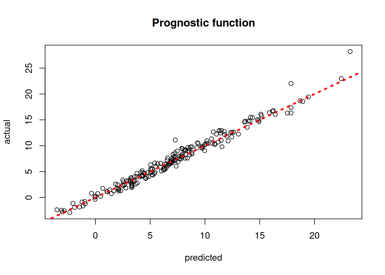

Python

mu_hat_test = bcf_model.predict(
    X=X_test, Z=Z_test, propensity=pi_test, terms="prognostic_function"
)
mu_pred = mu_hat_test.mean(axis=1)
lo, hi = min(mu_pred.min(), mu_test.min()), max(mu_pred.max(), mu_test.max())
plt.scatter(mu_pred, mu_test, alpha=0.5)
plt.plot([lo, hi], [lo, hi], color="red", linestyle="dashed", linewidth=2)
plt.xlabel("Predicted")
plt.ylabel("Actual")
plt.title("Prognostic function")
plt.show()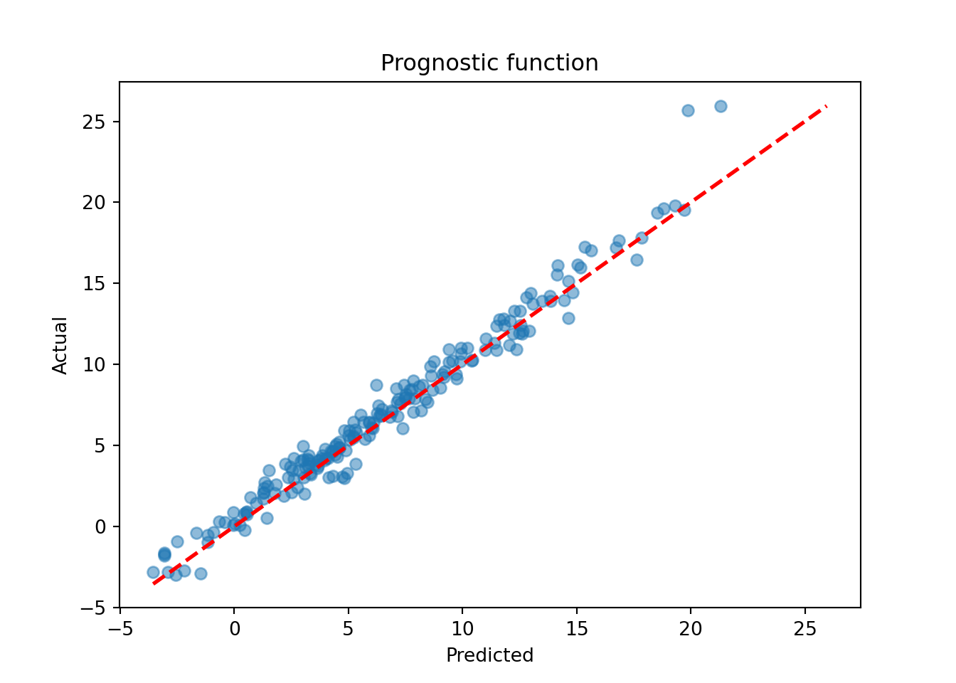

Plot the true versus estimated CATE function

R

tau_hat_test <- predict(
  bcf_model,
  X = X_test,
  Z = Z_test,
  propensity = pi_test,
  terms = "cate"
)
plot(
  rowMeans(tau_hat_test),
  tau_test,
  xlab = "predicted",
  ylab = "actual",
  main = "Treatment effect"
)
abline(0, 1, col = "red", lty = 3, lwd = 3)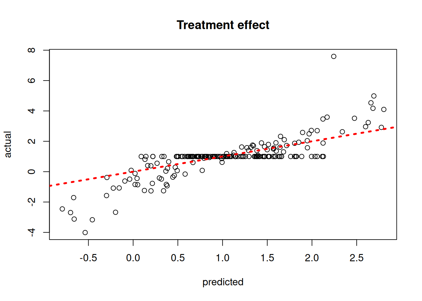

Python

tau_hat_test = bcf_model.predict(X=X_test, Z=Z_test, propensity=pi_test, terms="cate")
tau_pred = tau_hat_test.mean(axis=1)
lo, hi = min(tau_pred.min(), tau_test.min()), max(tau_pred.max(), tau_test.max())
plt.scatter(tau_pred, tau_test, alpha=0.5)
plt.plot([lo, hi], [lo, hi], color="red", linestyle="dashed", linewidth=2)
plt.xlabel("Predicted")
plt.ylabel("Actual")
plt.title("Treatment effect")
plt.show()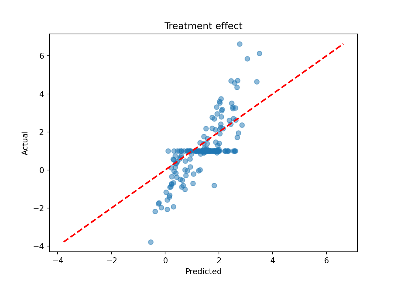

Plot the \(\sigma^2\) traceplot

R

sigma_observed <- var(y - E_XZ)
sigma2_global_samples <- extractParameter(bcf_model, "sigma2_global")
plot_bounds <- c(
  min(c(sigma2_global_samples, sigma_observed)),
  max(c(sigma2_global_samples, sigma_observed))
)
plot(
  sigma2_global_samples,
  ylim = plot_bounds,
  ylab = "sigma^2",
  xlab = "Sample",
  main = "Global variance parameter"
)
abline(h = sigma_observed, lty = 3, lwd = 3, col = "blue")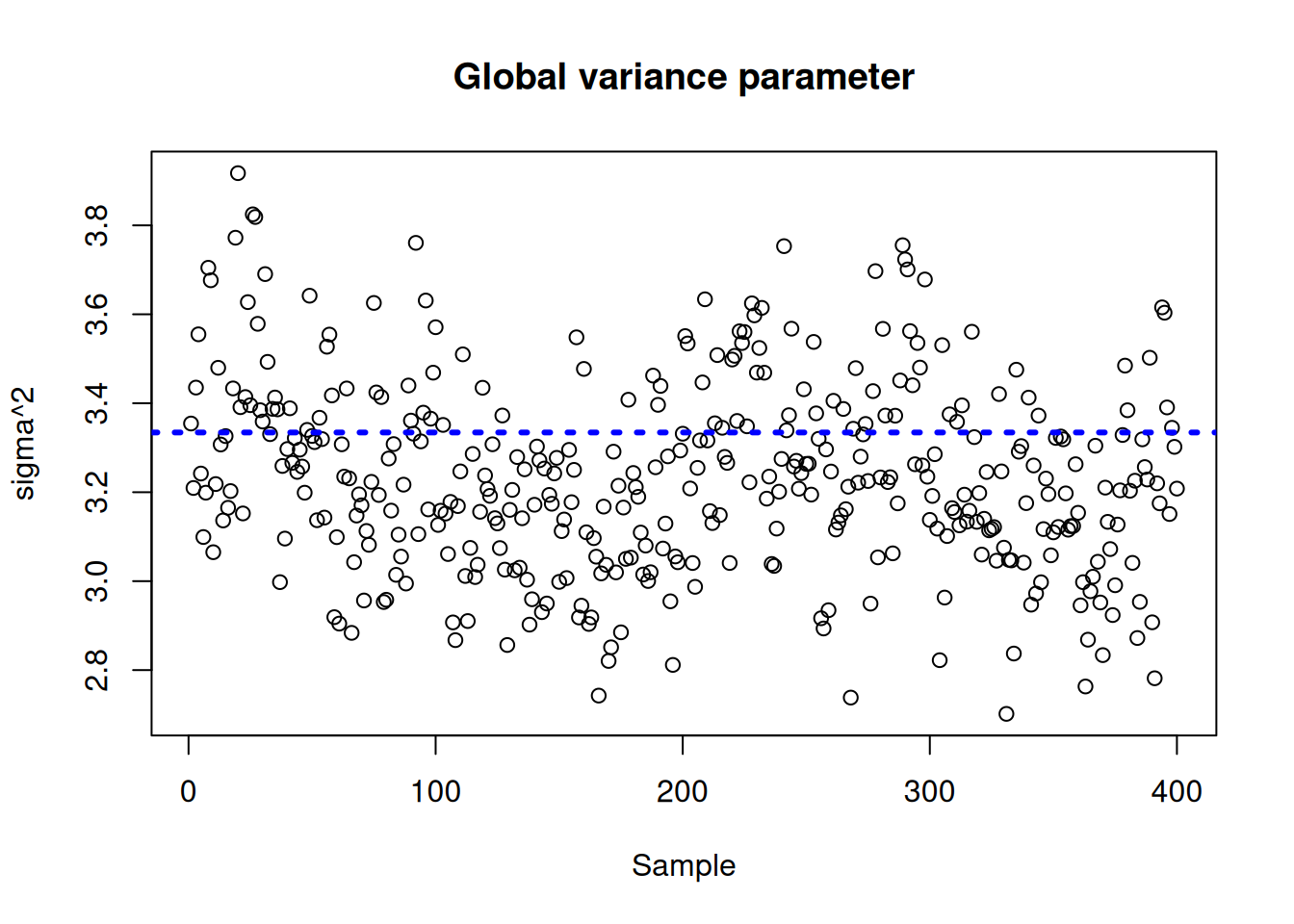

Python

sigma_observed = np.var(y - E_XZ)
global_var_samples = bcf_model.extract_parameter("sigma2_global")
plt.plot(global_var_samples)
plt.axhline(sigma_observed, color="blue", linestyle="dashed", linewidth=2)
plt.xlabel("Sample")
plt.ylabel(r"$\sigma^2$")
plt.title("Global variance parameter")
plt.show()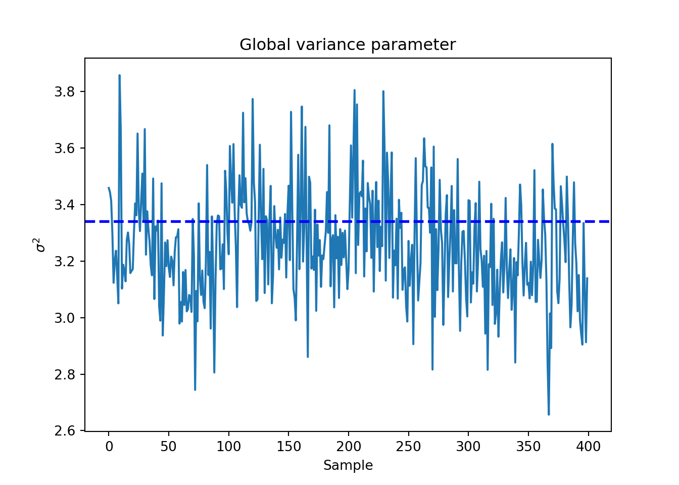

Examine test set interval coverage of \(\tau(X)\).

R

test_lb <- apply(tau_hat_test, 1, quantile, 0.025)
test_ub <- apply(tau_hat_test, 1, quantile, 0.975)
cover <- ((test_lb <= tau_x[test_inds]) &
  (test_ub >= tau_x[test_inds]))
cat("CATE function interval coverage: ", mean(cover) * 100, "%\n")

CATE function interval coverage:  92 %

Python

test_lb = np.quantile(tau_hat_test, 0.025, axis=1)
test_ub = np.quantile(tau_hat_test, 0.975, axis=1)
cover = (test_lb <= tau_test) & (test_ub >= tau_test)
print(f"CATE function interval coverage: {cover.mean() * 100:.2f}%")

CATE function interval coverage: 84.00%

References

Hahn, P Richard, Jared S Murray, and Carlos M Carvalho. 2020. “Bayesian Regression Tree Models for Causal Inference: Regularization, Confounding, and Heterogeneous Effects (with Discussion).” Bayesian Analysis 15 (3): 965–1056.

He, Jingyu, and P Richard Hahn. 2023. “Stochastic Tree Ensembles for Regularized Nonlinear Regression.” Journal of the American Statistical Association 118 (541): 551–70.

Krantsevich, Nikolay, Jingyu He, and P Richard Hahn. 2023. “Stochastic Tree Ensembles for Estimating Heterogeneous Effects.” International Conference on Artificial Intelligence and Statistics, 6120–31.