library(stochtree)BCF with Vector-valued Treatments
BCF extended to vector-valued (multivariate) treatments, estimating heterogeneous effects for multiple treatment arms simultaneously.
Background
When treatments are multivariate — such as continuous dose vectors or multiple binary arms — the standard BCF model extends to
\[ Y_i = \mu(X_i) + \tau(X_i)^\top Z_i + \epsilon_i \]
where \(Z_i \in \mathbb{R}^p\) and \(\tau(X_i) \in \mathbb{R}^p\) is a vector of covariate-dependent treatment effects.
Setup
Load necessary packages
import matplotlib.pyplot as plt
import numpy as np
from sklearn.model_selection import train_test_split
from stochtree import BCFModel
Set a seed for reproducibility
random_seed <- 4321
set.seed(random_seed)
random_seed = 4321
rng = np.random.default_rng(random_seed)Data Simulation
# Generate covariates, propensities, and treatments
n <- 1000
p_X <- 5
X <- matrix(runif(n * p_X), nrow = n, ncol = p_X)
pi_X <- cbind(0.25 + 0.5 * X[, 1], 0.75 - 0.5 * X[, 2])
Z <- cbind(
  as.numeric(rbinom(n, 1, pi_X[, 1])),
  as.numeric(rbinom(n, 1, pi_X[, 2]))
)

# Define outcome mean functions (prognostic and treatment effects)
mu_X <- pi_X[, 1] * 5 + pi_X[, 2] * 2 + 2 * X[, 3]
tau_X <- cbind(X[, 2], X[, 3])

# Generate outcome
treatment_term <- rowSums(tau_X * Z)
y <- mu_X + treatment_term + rnorm(n)
# Generate covariates, propensities, and treatments
n = 1000
p_X = 5
X = rng.uniform(0, 1, (n, p_X))
pi_X = np.c_[0.25 + 0.5 * X[:, 0], 0.75 - 0.5 * X[:, 1]]
Z = rng.binomial(1, pi_X, (n, 2)).astype(float)
# Define the outcome mean functions (prognostic and treatment effects)
mu_X = pi_X[:, 0] * 5 + pi_X[:, 1] * 2 + 2 * X[:, 2]
tau_X = np.stack((X[:, 1], X[:, 2]), axis=-1)
# Generate outcome
epsilon = rng.normal(0, 1, n)
treatment_term = np.multiply(tau_X, Z).sum(axis=1)
y = mu_X + treatment_term + epsilonSplit the data into train and test sets
n_test <- round(n * 0.2)
test_inds <- sort(sample(seq_len(n), n_test, replace = FALSE))
train_inds <- setdiff(seq_len(n), test_inds)
X_train <- X[train_inds, ]
X_test <- X[test_inds, ]
Z_train <- Z[train_inds, ]
Z_test <- Z[test_inds, ]
y_train <- y[train_inds]
y_test <- y[test_inds]
pi_train <- pi_X[train_inds, ]
pi_test <- pi_X[test_inds, ]
mu_train <- mu_X[train_inds]
mu_test <- mu_X[test_inds]
tau_train <- tau_X[train_inds, ]
tau_test <- tau_X[test_inds, ]
sample_inds = np.arange(n)
train_inds, test_inds = train_test_split(sample_inds, test_size=0.2)
X_train = X[train_inds, :]
X_test = X[test_inds, :]
Z_train = Z[train_inds, :]
Z_test = Z[test_inds, :]
y_train = y[train_inds]
y_test = y[test_inds]
pi_train = pi_X[train_inds]
pi_test = pi_X[test_inds]
mu_train = mu_X[train_inds]
mu_test = mu_X[test_inds]
tau_train = tau_X[train_inds, :]
tau_test = tau_X[test_inds, :]Model Fitting
Fit a multivariate BCF model
general_params <- list(
  num_threads = 1,
  num_chains = 4,
  random_seed = random_seed,
  adaptive_coding = FALSE
)
bcf_model <- bcf(
  X_train = X_train,
  Z_train = Z_train,
  y_train = y_train,
  propensity_train = pi_train,
  num_gfr = 10,
  num_burnin = 500,
  num_mcmc = 100,
  general_params = general_params
)
general_params = {
"num_threads": 1,
"num_chains": 4,
"random_seed": random_seed,
"adaptive_coding": False
}
bcf_model = BCFModel()
bcf_model.sample(
X_train=X_train,
Z_train=Z_train,
y_train=y_train,
propensity_train=pi_train,
num_gfr=10,
num_burnin=500,
num_mcmc=100,
general_params=general_params,
)Posterior Summaries
Compare true outcomes to predicted conditional means
y_hat_test <- predict(
  bcf_model,
  X = X_test,
  Z = Z_test,
  propensity = pi_test,
  terms = "y_hat",
  type = "mean"
)
plot(
  y_hat_test,
  y_test,
  xlab = "Average estimated outcome",
  ylab = "True outcome"
)
abline(0, 1, col = "black", lty = 3)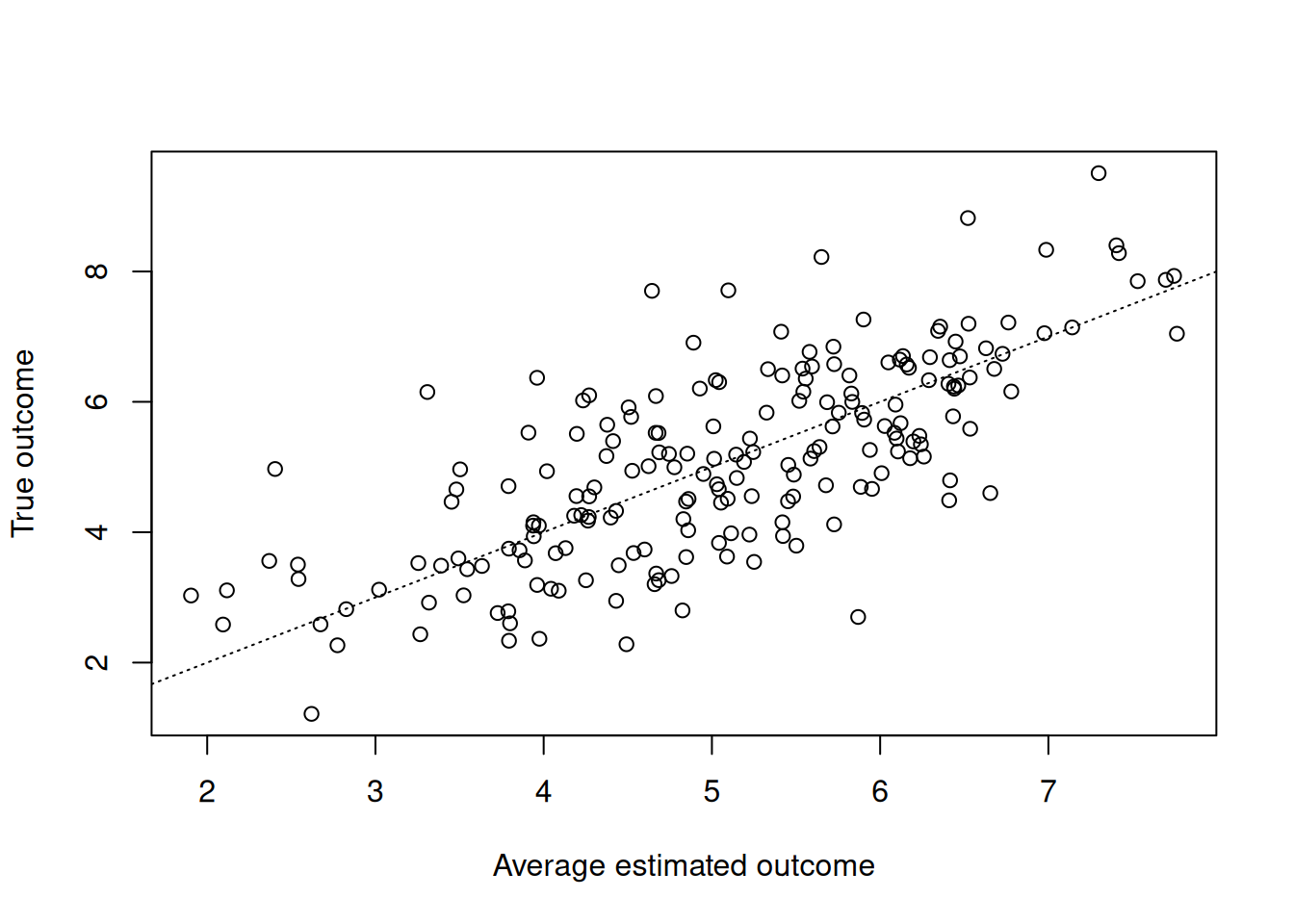
rmse <- sqrt(mean((y_hat_test - y_test)^2))
cat("Test-set RMSE: ", rmse, "\n")
Test-set RMSE: 1.039821 y_hat_test = bcf_model.predict(
X=X_test, Z=Z_test, propensity=pi_test, terms="y_hat", type="mean"
)
lo, hi = min(y_hat_test.min(), y_test.min()), max(y_hat_test.max(), y_test.max())
plt.scatter(y_hat_test, y_test, alpha=0.5)
plt.plot([lo, hi], [lo, hi], color="red", linestyle="dashed", linewidth=2)
plt.xlabel("Predicted")
plt.ylabel("Actual")
plt.title("Outcome")
plt.show()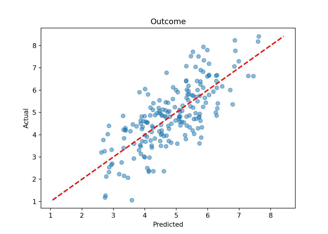
rmse = np.sqrt(np.mean(np.power(y_hat_test - y_test, 2)))
print(f"Test-set RMSE: {rmse:.2f}")
Test-set RMSE: 1.06Compare true versus estimated treatment effects for each treatment entry
tau_hat_test <- predict(
  bcf_model,
  X = X_test,
  Z = Z_test,
  propensity = pi_test,
  terms = "cate",
  type = "mean"
)
plot(
  tau_test[, 1],
  tau_hat_test[, 1],
  xlab = "True tau",
  ylab = "Average estimated tau",
  main = "Treatment 1"
)
abline(0, 1, col = "black", lty = 3)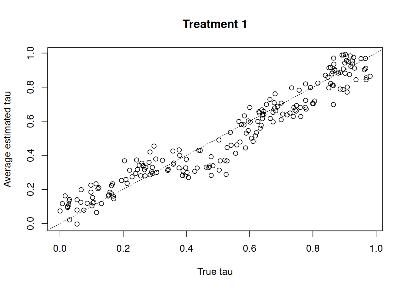
plot(
  tau_test[, 2],
  tau_hat_test[, 2],
  xlab = "True tau",
  ylab = "Average estimated tau",
  main = "Treatment 2"
)
abline(0, 1, col = "black", lty = 3)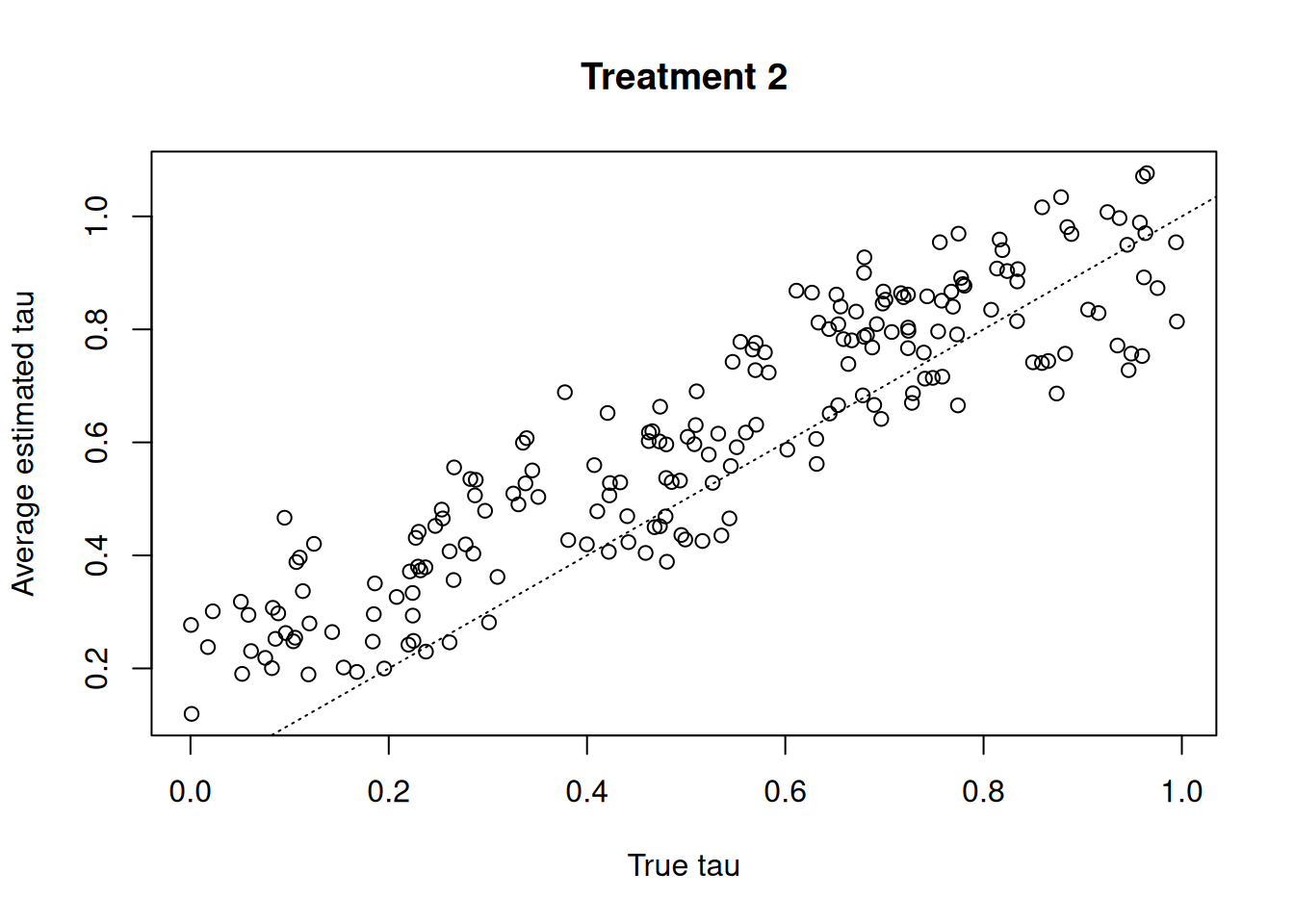
tau_hat_test = bcf_model.predict(
    X=X_test, Z=Z_test, propensity=pi_test, terms="cate", type="mean"
)
treatment_idx = 0
lo, hi = (
    min((tau_hat_test[:, treatment_idx]).min(), (tau_test[:, treatment_idx]).min()),
    max((tau_hat_test[:, treatment_idx]).max(), (tau_test[:, treatment_idx]).max()),
)
plt.scatter(tau_test[:, treatment_idx], tau_hat_test[:, treatment_idx], alpha=0.5)
plt.plot([lo, hi], [lo, hi], color="red", linestyle="dashed", linewidth=2)
plt.xlabel("True tau")
plt.ylabel("Average estimated tau")
plt.title(f"Treatment {treatment_idx + 1}")
plt.show()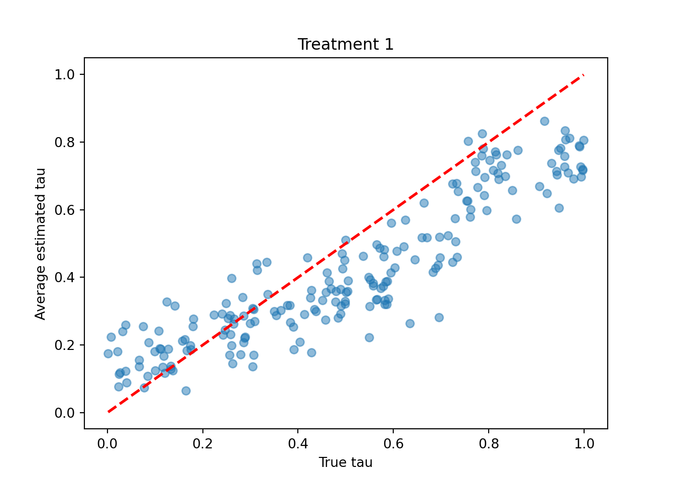
treatment_idx = 1
lo, hi = (
    min((tau_hat_test[:, treatment_idx]).min(), (tau_test[:, treatment_idx]).min()),
    max((tau_hat_test[:, treatment_idx]).max(), (tau_test[:, treatment_idx]).max()),
)
plt.scatter(tau_test[:, treatment_idx], tau_hat_test[:, treatment_idx], alpha=0.5)
plt.plot([lo, hi], [lo, hi], color="red", linestyle="dashed", linewidth=2)
plt.xlabel("True tau")
plt.ylabel("Average estimated tau")
plt.title(f"Treatment {treatment_idx + 1}")
plt.show()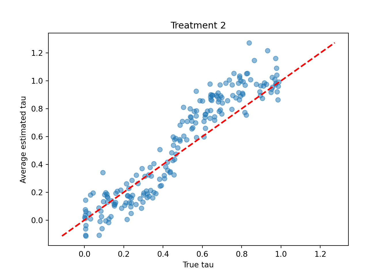
Now compare the true versus estimated treatment terms of the model (i.e. \(t_i = \sum_j(\tau_{i,j}(X) * Z_{i,j})\) where \(i\) indexes observations and \(j\) indexes treatments)
tau_hat_test <- predict(
  bcf_model,
  X = X_test,
  Z = Z_test,
  propensity = pi_test,
  terms = "cate",
  type = "posterior"
)
treatment_term_mcmc <- apply(tau_hat_test, 3, function(tau_s) {
  rowSums(tau_s * Z_test)
})
true_treatment_term <- rowSums(tau_test * Z_test)
plot(
  true_treatment_term,
  rowMeans(treatment_term_mcmc),
  xlab = "True treatment term",
  ylab = "Average estimated treatment term"
)
abline(0, 1, col = "black", lty = 3)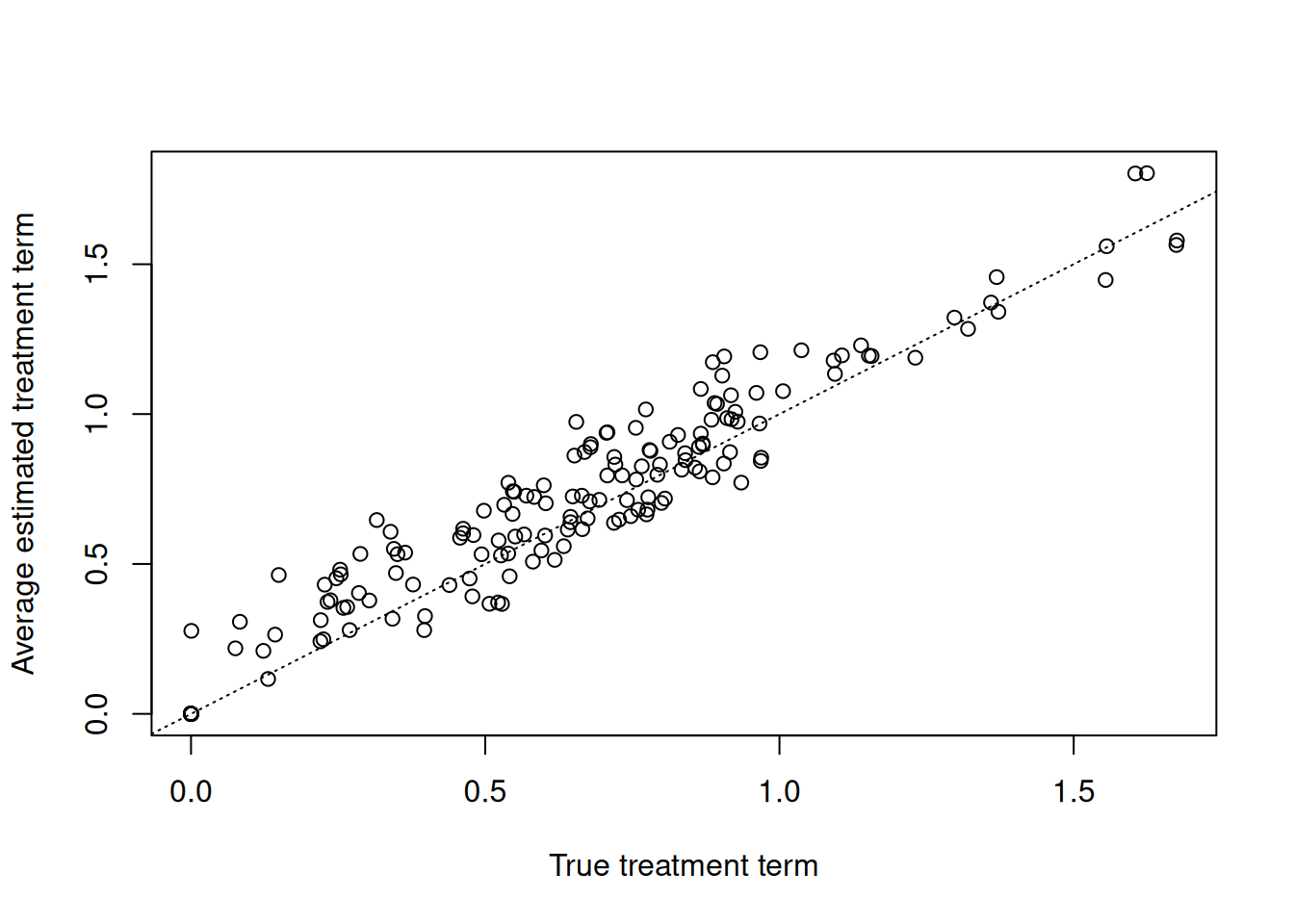
tau_hat_test = bcf_model.predict(
    X=X_test, Z=Z_test, propensity=pi_test, terms="cate", type="posterior"
)
treatment_term_mcmc_test = np.multiply(
    np.atleast_3d(Z_test).swapaxes(1, 2), tau_hat_test
).sum(axis=2)
treatment_term_test = np.multiply(tau_test, Z_test).sum(axis=1)
treatment_term_hat_test = np.squeeze(treatment_term_mcmc_test).mean(
    axis=1, keepdims=True
)
lo, hi = (
    min((treatment_term_hat_test).min(), (treatment_term_test).min()),
    max((treatment_term_hat_test).max(), (treatment_term_test).max()),
)
plt.scatter(treatment_term_test, treatment_term_hat_test, alpha=0.5)
plt.plot([lo, hi], [lo, hi], color="red", linestyle="dashed", linewidth=2)
plt.xlabel("True value")
plt.ylabel("Average estimated value")
plt.title("Treatment Term")
plt.show()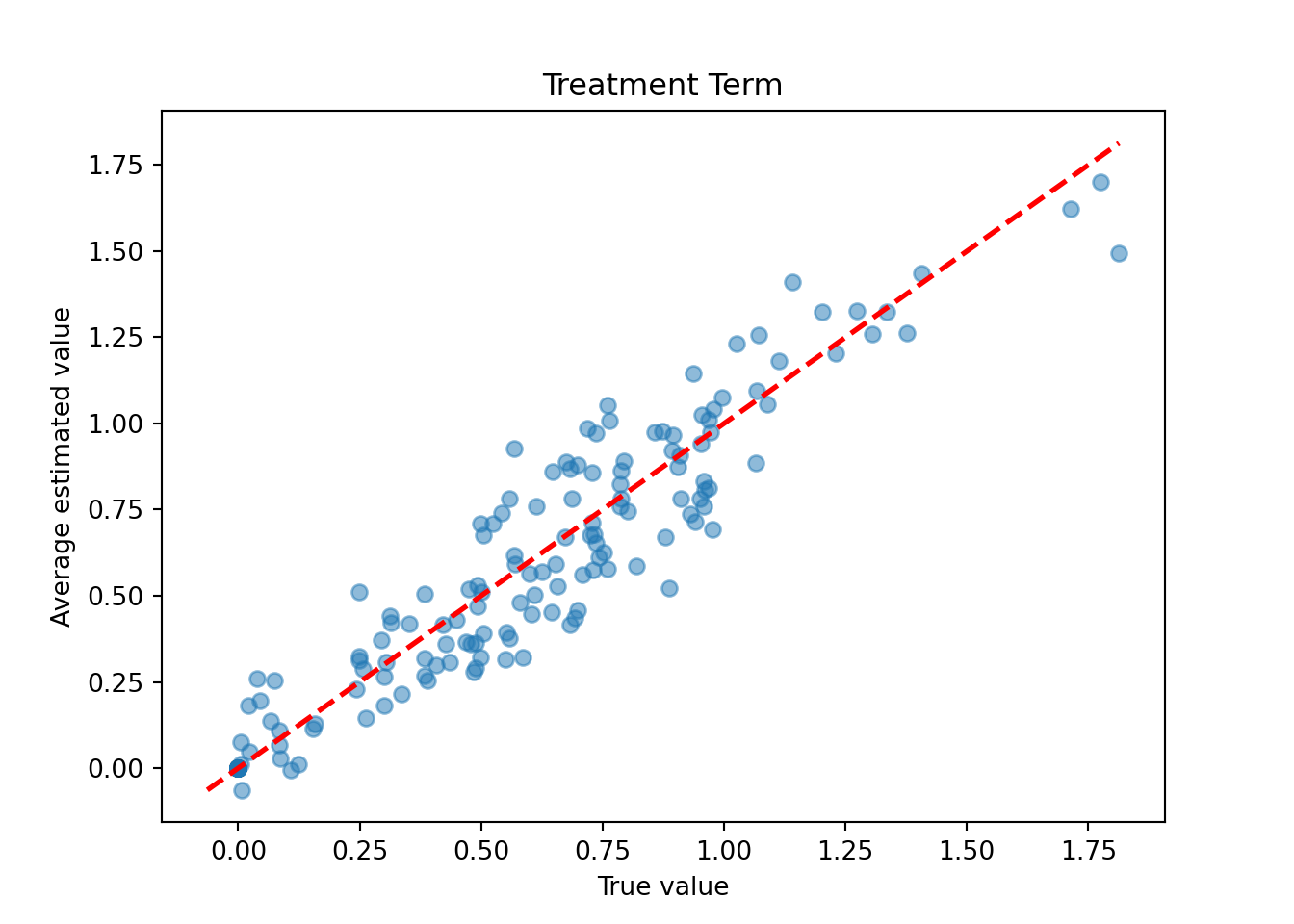
Compare true and predicted prognostic function values
mu_hat_test <- predict(
  bcf_model,
  X = X_test,
  Z = Z_test,
  propensity = pi_test,
  terms = "prognostic_function",
  type = "mean"
)
plot(
  mu_test,
  mu_hat_test,
  xlab = "True value",
  ylab = "Average estimated value",
  main = "Prognostic Function"
)
abline(0, 1, col = "black", lty = 3)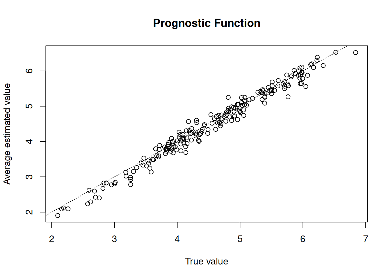
mu_hat_test = bcf_model.predict(
    X=X_test, Z=Z_test, propensity=pi_test, terms="prognostic_function", type="mean"
)
lo, hi = (
    min((mu_hat_test).min(), (mu_test).min()),
    max((mu_hat_test).max(), (mu_test).max()),
)
plt.scatter(mu_hat_test, mu_test, alpha=0.5)
plt.plot([lo, hi], [lo, hi], color="red", linestyle="dashed", linewidth=2)
plt.xlabel("True value")
plt.ylabel("Average estimated value")
plt.title("Prognostic Function")
plt.show()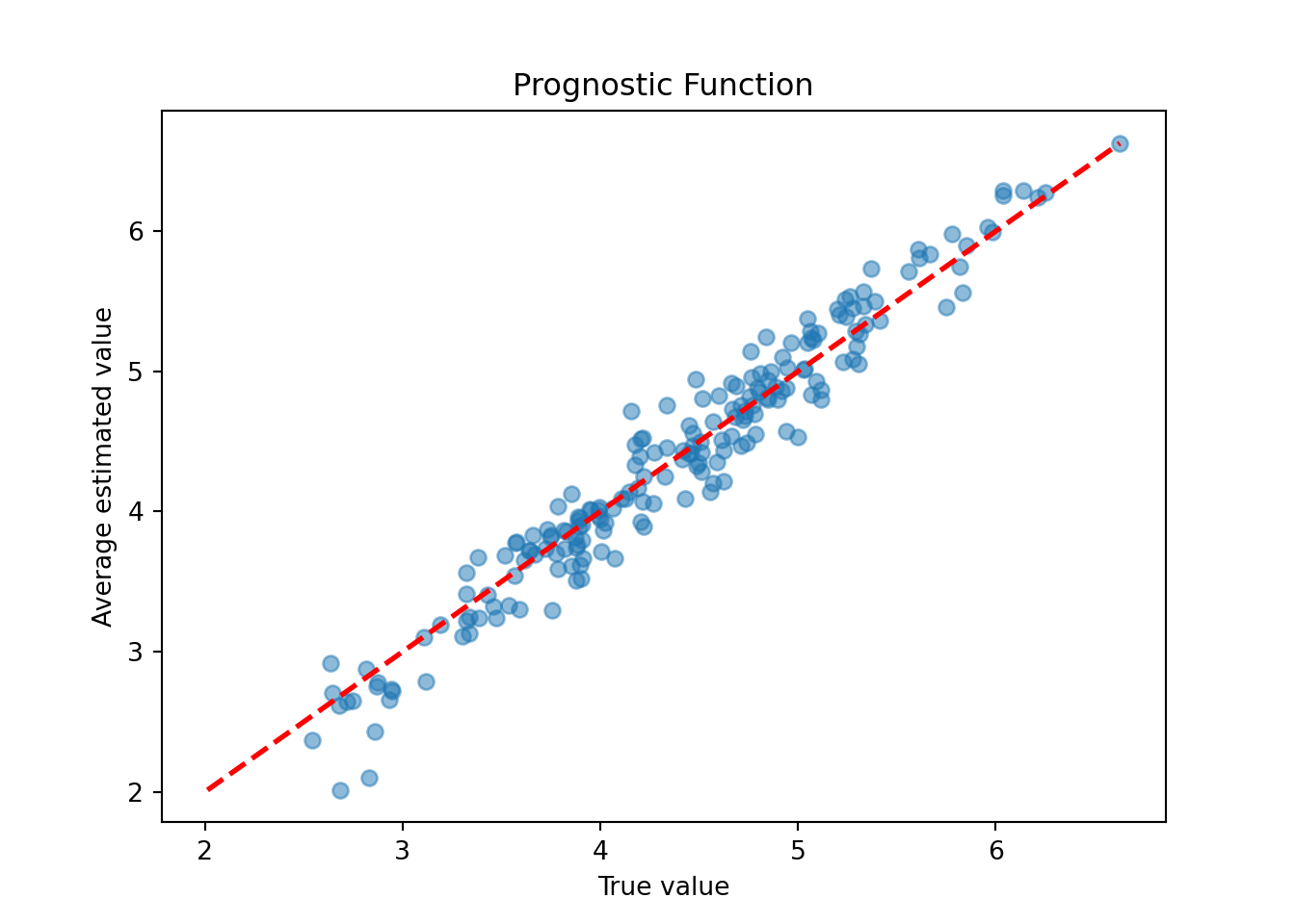
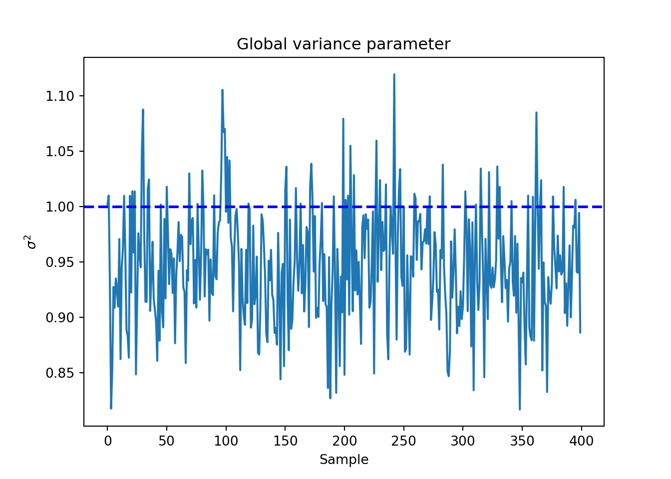
Finally, we inspect the traceplot of the global error variance, \(\sigma^2\)
sigma2_global_samples <- extractParameter(bcf_model, "sigma2_global")
plot(
  sigma2_global_samples,
  xlab = "Sample",
  ylab = expression(sigma^2)
)
abline(h = 1, lty = 3, lwd = 3, col = "blue")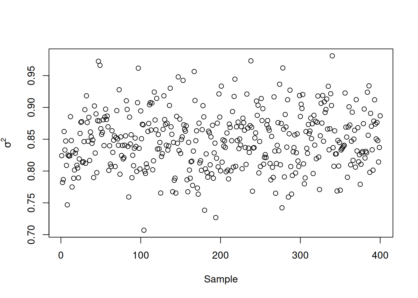
global_var_samples = bcf_model.extract_parameter("sigma2_global")
plt.plot(global_var_samples)
plt.axhline(1, color="blue", linestyle="dashed", linewidth=2)
plt.xlabel("Sample")
plt.ylabel(r"$\sigma^2$")
plt.title("Global variance parameter")
plt.show()