Using Shared Leaf Membership as a Kernel

A trained tree ensemble with strong out-of-sample performance admits a natural motivation for the “distance” between two samples: shared leaf membership. This vignette demonstrates how to extract a kernel matrix from a fitted stochtree ensemble and use it for Gaussian process inference.

Motivation

We number the leaves in an ensemble from 1 to \(s\) (that is, if tree 1 has 3 leaves, it reserves the numbers 1 - 3, and in turn if tree 2 has 5 leaves, it reserves the numbers 4 - 8 to label its leaves, and so on). For a dataset with \(n\) observations, we construct the matrix \(W\) as follows:

Initialize \(W\) as a matrix of all zeroes with \(n\) rows and as many columns as leaves in the ensemble

Let s = 0

For \(j\) in \(\left\{1,\dots,m\right\}\):

Let num_leaves be the number of leaves in tree \(j\)

For \(i\) in \(\left\{1,\dots,n\right\}\):

Let k be the leaf to which tree \(j\) maps observation \(i\)

Set element \(W_{i,k+s} = 1\)

Let s = s + num_leaves

This sparse matrix \(W\) is a matrix representation of the basis predictions of an ensemble (i.e. integrating out the leaf parameters and just analyzing the leaf indices). For an ensemble with \(m\) trees, we can determine the proportion of trees that map each observation to the same leaf by computing \(W W^T / m\). This can form the basis for a kernel function used in a Gaussian process regression, as we demonstrate below.

Setup

Load necessary packages

library(stochtree)
library(tgp)
library(MASS)
library(Matrix)
library(mvtnorm)

import numpy as np
import matplotlib.pyplot as plt
from scipy.sparse import csr_matrix
from sklearn.gaussian_process import GaussianProcessRegressor
from sklearn.gaussian_process.kernels import RBF, WhiteKernel
from sklearn.datasets import make_friedman1

from stochtree import BARTModel, compute_forest_leaf_indices

Set a seed for reproducibility

random_seed <- 101
set.seed(random_seed)

random_seed = 101
rng = np.random.default_rng(random_seed)

Demo 1: Univariate Supervised Learning

We begin with a non-stationary simulated DGP with a single numeric covariate, originally described in Gramacy and Taddy (2010). We define a training set and test set and evaluate various approaches to modeling the out-of-sample outcome.

Traditional Gaussian Process

# Generate the data
X_train <- seq(0,20,length=100)
X_test <- seq(0,20,length=99)
y_train <- (sin(pi*X_train/5) + 0.2*cos(4*pi*X_train/5)) * (X_train <= 9.6)
lin_train <- X_train>9.6;
y_train[lin_train] <- -1 + X_train[lin_train]/10
y_train <- y_train + rnorm(length(y_train), sd=0.1)
y_test <- (sin(pi*X_test/5) + 0.2*cos(4*pi*X_test/5)) * (X_test <= 9.6)
lin_test <- X_test>9.6;
y_test[lin_test] <- -1 + X_test[lin_test]/10

# Fit the GP
model_gp <- bgp(X=X_train, Z=y_train, XX=X_test)
plot(model_gp$ZZ.mean, y_test, xlab = "predicted", ylab = "actual", main = "Gaussian process")
abline(0,1,lwd=2.5,lty=3,col="red")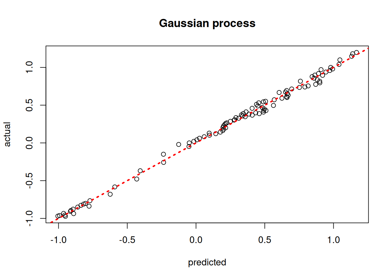

# Generate the data
X_train_1d = np.linspace(0, 20, 100)
X_test_1d  = np.linspace(0, 20, 99)

y_train_1 = (np.sin(np.pi * X_train_1d / 5) + 0.2 * np.cos(4 * np.pi * X_train_1d / 5)) * (X_train_1d <= 9.6)
y_train_1[X_train_1d > 9.6] = -1 + X_train_1d[X_train_1d > 9.6] / 10
y_train_1 = y_train_1 + rng.normal(0, 0.1, len(X_train_1d))

y_test_1 = (np.sin(np.pi * X_test_1d / 5) + 0.2 * np.cos(4 * np.pi * X_test_1d / 5)) * (X_test_1d <= 9.6)
y_test_1[X_test_1d > 9.6] = -1 + X_test_1d[X_test_1d > 9.6] / 10

# sklearn's GaussianProcessRegressor is used here in place of R's tgp::bgp
X_train_2d = X_train_1d.reshape(-1, 1)
X_test_2d  = X_test_1d.reshape(-1, 1)
gp_kernel = RBF(length_scale=1.0) + WhiteKernel(noise_level=0.01)
model_gp_1 = GaussianProcessRegressor(kernel=gp_kernel, n_restarts_optimizer=5,
                                       random_state=random_seed)
model_gp_1.fit(X_train_2d, y_train_1)

GaussianProcessRegressor(kernel=RBF(length_scale=1) + WhiteKernel(noise_level=0.01),
                         n_restarts_optimizer=5, random_state=101)

In a Jupyter environment, please rerun this cell to show the HTML representation or trust the notebook.
On GitHub, the HTML representation is unable to render, please try loading this page with nbviewer.org.

gp_pred_1 = model_gp_1.predict(X_test_2d)

plt.scatter(gp_pred_1, y_test_1, alpha=0.5)
lo, hi = min(gp_pred_1.min(), y_test_1.min()), max(gp_pred_1.max(), y_test_1.max())
plt.plot([lo, hi], [lo, hi], color="red", linestyle="dashed", linewidth=2)
plt.xlabel("Predicted")
plt.ylabel("Actual")
plt.title("Gaussian process")
plt.show()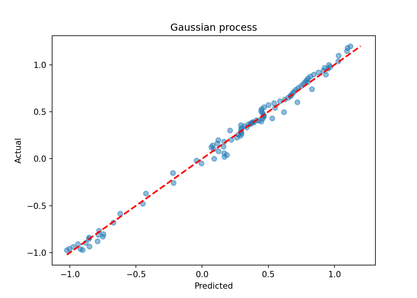

Assess the RMSE

sqrt(mean((model_gp$ZZ.mean - y_test)^2))

[1] 0.04299507

print(f"RMSE: {np.sqrt(np.mean((gp_pred_1 - y_test_1)**2)):.4f}")

RMSE: 0.0529

BART-based Gaussian Process

# Run BART on the data
num_trees <- 200
sigma_leaf <- 1/num_trees
X_train <- as.data.frame(X_train)
X_test <- as.data.frame(X_test)
colnames(X_train) <- colnames(X_test) <- "x1"
general_params <- list(num_threads=1)
mean_forest_params <- list(num_trees=num_trees, sigma2_leaf_init=sigma_leaf)
bart_model <- bart(X_train=X_train, y_train=y_train, X_test=X_test, 
                   general_params = general_params, mean_forest_params = mean_forest_params)

# Extract kernels needed for kriging
leaf_mat_train <- computeForestLeafIndices(bart_model, X_train, forest_type = "mean",
                                           forest_inds = bart_model$model_params$num_samples - 1)
leaf_mat_test <- computeForestLeafIndices(bart_model, X_test, forest_type = "mean",
                                           forest_inds = bart_model$model_params$num_samples - 1)
W_train <- sparseMatrix(i=rep(1:length(y_train),num_trees), j=leaf_mat_train + 1, x=1)
W_test <- sparseMatrix(i=rep(1:length(y_test),num_trees), j=leaf_mat_test + 1, x=1)
Sigma_11 <- tcrossprod(W_test) / num_trees
Sigma_12 <- tcrossprod(W_test, W_train) / num_trees
Sigma_22 <- tcrossprod(W_train) / num_trees
Sigma_22_inv <- ginv(as.matrix(Sigma_22))
Sigma_21 <- t(Sigma_12)

# Compute mean and covariance for the test set posterior
mu_tilde <- Sigma_12 %*% Sigma_22_inv %*% y_train
Sigma_tilde <- as.matrix((sigma_leaf)*(Sigma_11 - Sigma_12 %*% Sigma_22_inv %*% Sigma_21))

# Sample from f(X_test) | X_test, X_train, f(X_train)
gp_samples <- mvtnorm::rmvnorm(1000, mean = mu_tilde, sigma = Sigma_tilde)

# Compute posterior mean predictions for f(X_test)
yhat_mean_test <- colMeans(gp_samples)
plot(yhat_mean_test, y_test, xlab = "predicted", ylab = "actual", main = "BART Gaussian process")
abline(0,1,lwd=2.5,lty=3,col="red")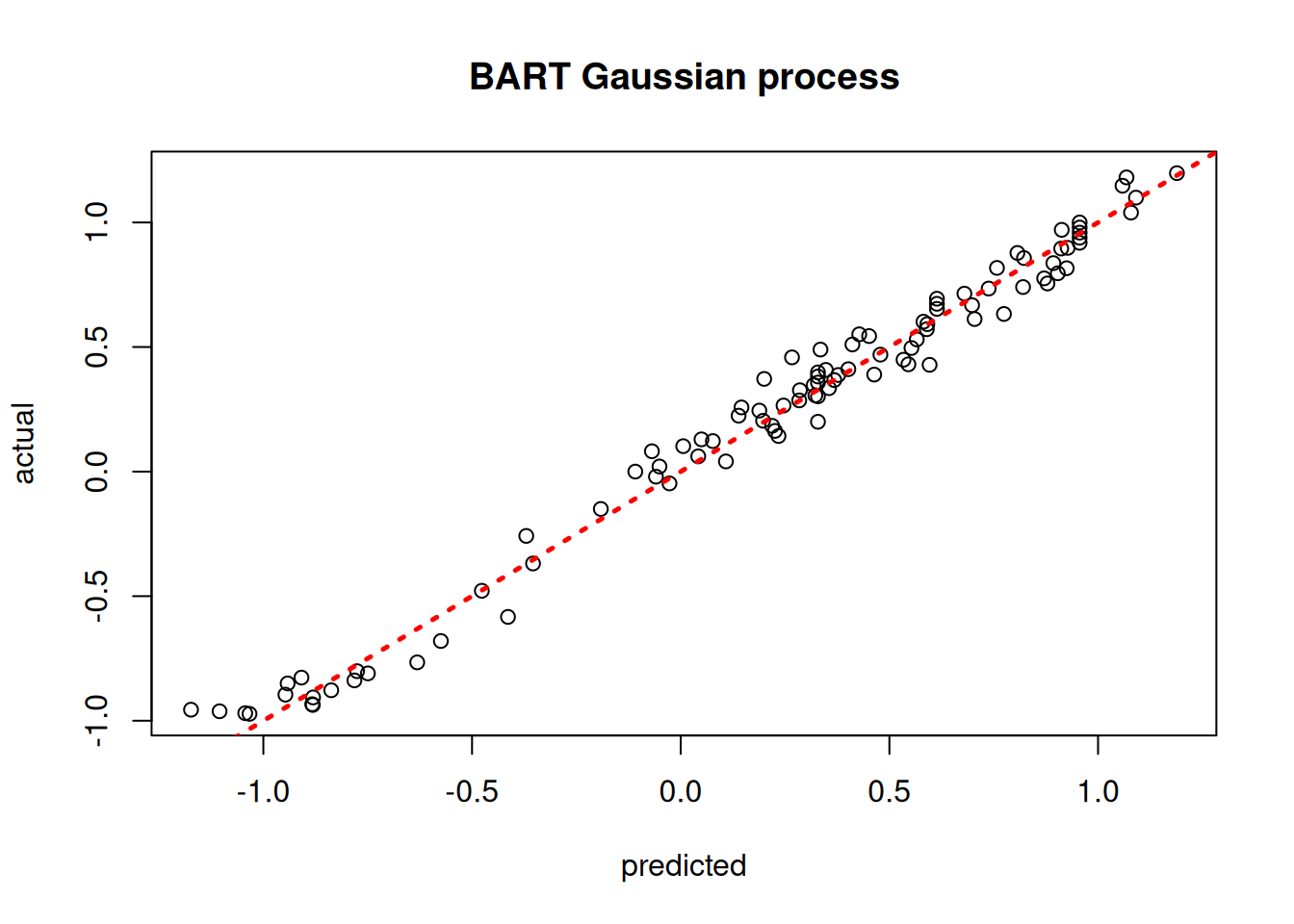

# Run BART on the data
num_trees = 200
sigma_leaf = 1 / num_trees
general_params = {"num_threads": 1}
mean_forest_params = {"num_trees": num_trees, "sigma2_leaf_init": sigma_leaf}
bart_model_1 = BARTModel()
bart_model_1.sample(X_train=X_train_2d, y_train=y_train_1, X_test=X_test_2d,
                    general_params=general_params, mean_forest_params=mean_forest_params)

# Extract leaf indices for the last retained forest sample
last_sample = bart_model_1.num_samples - 1
leaf_mat_train_1 = compute_forest_leaf_indices(bart_model_1, X_train_2d,
                                               forest_type="mean", forest_inds=last_sample)
leaf_mat_test_1  = compute_forest_leaf_indices(bart_model_1, X_test_2d,
                                               forest_type="mean", forest_inds=last_sample)

# Build sparse W matrices (rows = observations, cols = global leaf indices)
n_train_1, n_test_1 = len(y_train_1), len(y_test_1)
col_inds_train = leaf_mat_train_1.flatten()
col_inds_test  = leaf_mat_test_1.flatten()
max_col = max(col_inds_train.max(), col_inds_test.max()) + 1
W_train_1 = csr_matrix(
    (np.ones(len(col_inds_train)), (np.tile(np.arange(n_train_1), num_trees), col_inds_train)),
    shape=(n_train_1, max_col),
)
W_test_1 = csr_matrix(
    (np.ones(len(col_inds_test)), (np.tile(np.arange(n_test_1), num_trees), col_inds_test)),
    shape=(n_test_1, max_col),
)

# Compute kernel matrices
W_tr = W_train_1.toarray()
W_te = W_test_1.toarray()
Sigma_22   = (W_tr @ W_tr.T) / num_trees
Sigma_11   = (W_te @ W_te.T) / num_trees
Sigma_12   = (W_te @ W_tr.T) / num_trees
Sigma_21   = Sigma_12.T
Sigma_22_inv = np.linalg.pinv(Sigma_22)

# Compute GP posterior mean and covariance
mu_tilde    = Sigma_12 @ Sigma_22_inv @ y_train_1
Sigma_tilde = sigma_leaf * (Sigma_11 - Sigma_12 @ Sigma_22_inv @ Sigma_21)
Sigma_tilde += 1e-8 * np.eye(n_test_1)  # small jitter for numerical stability

# Sample from f(X_test) | X_test, X_train, f(X_train)
gp_samples_1 = rng.multivariate_normal(mu_tilde, Sigma_tilde, size=1000, method="eigh")

# Posterior mean predictions
yhat_mean_test_1 = gp_samples_1.mean(axis=0)
lo = min(yhat_mean_test_1.min(), y_test_1.min())
hi = max(yhat_mean_test_1.max(), y_test_1.max())
plt.scatter(yhat_mean_test_1, y_test_1, alpha=0.5)
plt.plot([lo, hi], [lo, hi], color="red", linestyle="dashed", linewidth=2)
plt.xlabel("Predicted")
plt.ylabel("Actual")
plt.title("BART Gaussian process")
plt.show()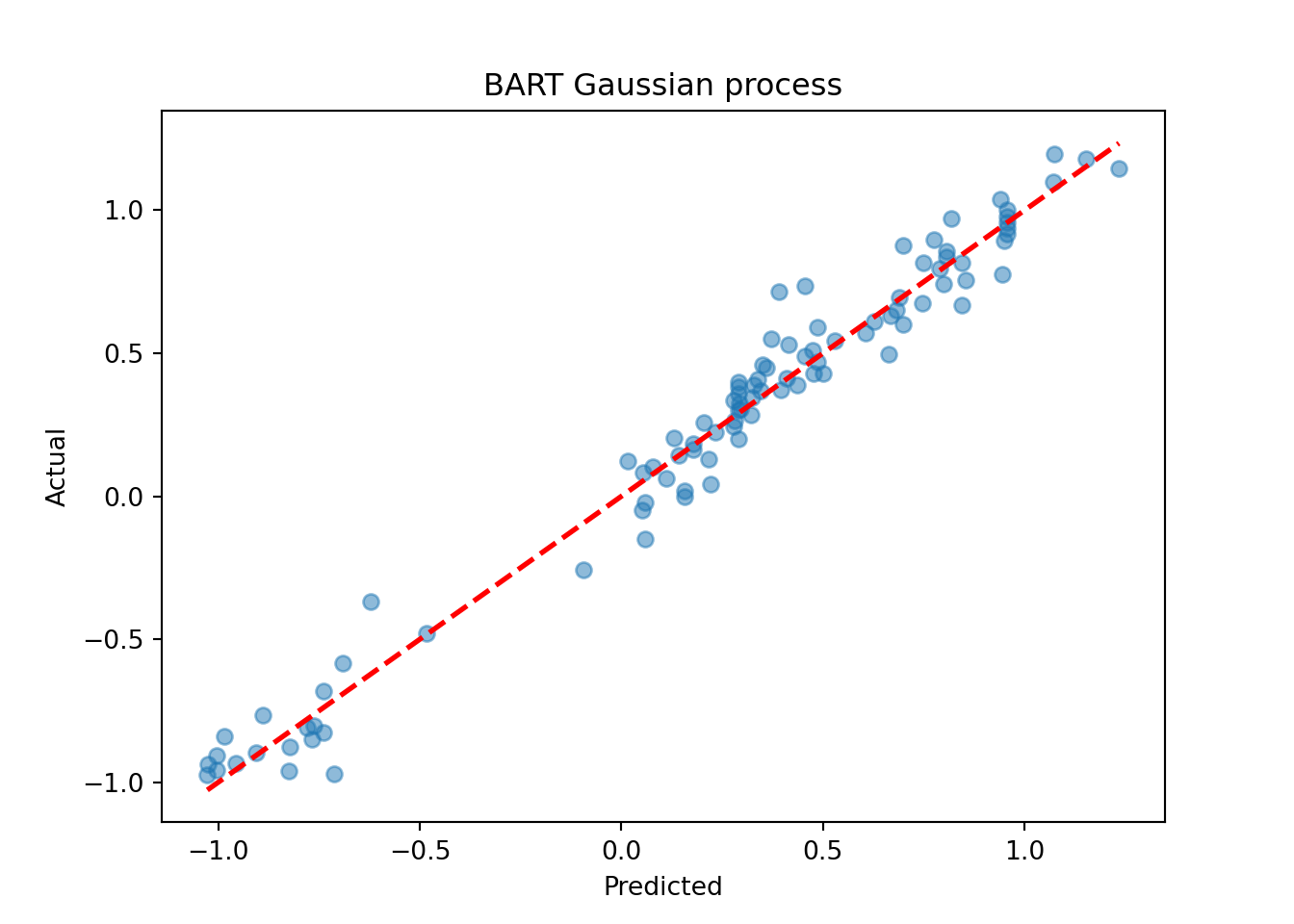

Assess the RMSE

sqrt(mean((yhat_mean_test - y_test)^2))

[1] 0.08037617

print(f"RMSE: {np.sqrt(np.mean((yhat_mean_test_1 - y_test_1)**2)):.4f}")

RMSE: 0.1003

Demo 2: Multivariate Supervised Learning

We proceed to the simulated “Friedman” dataset (Friedman (1991)). In R, this is accessed via tgp::friedman.1.data; in Python we use sklearn.datasets.make_friedman1, which implements the same DGP.

Traditional Gaussian Process

# Generate the data, add many "noise variables"
n <- 100
friedman.df <- friedman.1.data(n=n)
train_inds <- sort(sample(1:n, floor(0.8*n), replace = FALSE))
test_inds <- (1:n)[!((1:n) %in% train_inds)]
X <- as.matrix(friedman.df)[,1:10]
X <- cbind(X, matrix(runif(n*10), ncol = 10))
y <- as.matrix(friedman.df)[,12] + rnorm(n,0,1)*(sd(as.matrix(friedman.df)[,11])/2)
X_train <- X[train_inds,]
X_test <- X[test_inds,]
y_train <- y[train_inds]
y_test <- y[test_inds]

# Fit the GP
model_gp <- bgp(X=X_train, Z=y_train, XX=X_test)
plot(model_gp$ZZ.mean, y_test, xlab = "predicted", ylab = "actual", main = "Gaussian process")
abline(0,1,lwd=2.5,lty=3,col="red")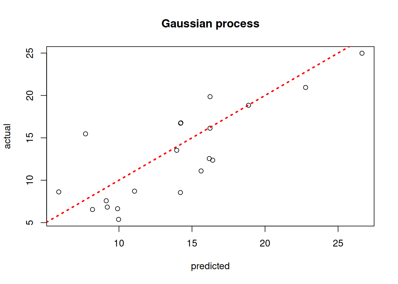

# Generate the data: 10 Friedman features + 10 noise features
n = 100
X_raw, y_friedman = make_friedman1(n_samples=n, n_features=10, noise=1.0,
                                    random_state=random_seed)
X_2 = np.hstack([X_raw, rng.uniform(size=(n, 10))])  # 20 features total
y_2 = y_friedman

train_inds_2 = rng.choice(n, int(0.8 * n), replace=False)
test_inds_2  = np.setdiff1d(np.arange(n), train_inds_2)
X_train_2, X_test_2 = X_2[train_inds_2], X_2[test_inds_2]
y_train_2, y_test_2 = y_2[train_inds_2], y_2[test_inds_2]

# sklearn's GaussianProcessRegressor is used here in place of R's tgp::bgp
gp_kernel_2 = RBF(length_scale=1.0) + WhiteKernel(noise_level=1.0)
model_gp_2 = GaussianProcessRegressor(kernel=gp_kernel_2, n_restarts_optimizer=1,
                                       random_state=random_seed)
model_gp_2.fit(X_train_2, y_train_2)

GaussianProcessRegressor(kernel=RBF(length_scale=1) + WhiteKernel(noise_level=1),
                         n_restarts_optimizer=1, random_state=101)

gp_pred_2 = model_gp_2.predict(X_test_2)

lo = min(gp_pred_2.min(), y_test_2.min())
hi = max(gp_pred_2.max(), y_test_2.max())
plt.scatter(gp_pred_2, y_test_2, alpha=0.6)
plt.plot([lo, hi], [lo, hi], color="red", linestyle="dashed", linewidth=2)
plt.xlabel("Predicted")
plt.ylabel("Actual")
plt.title("Gaussian process")
plt.show()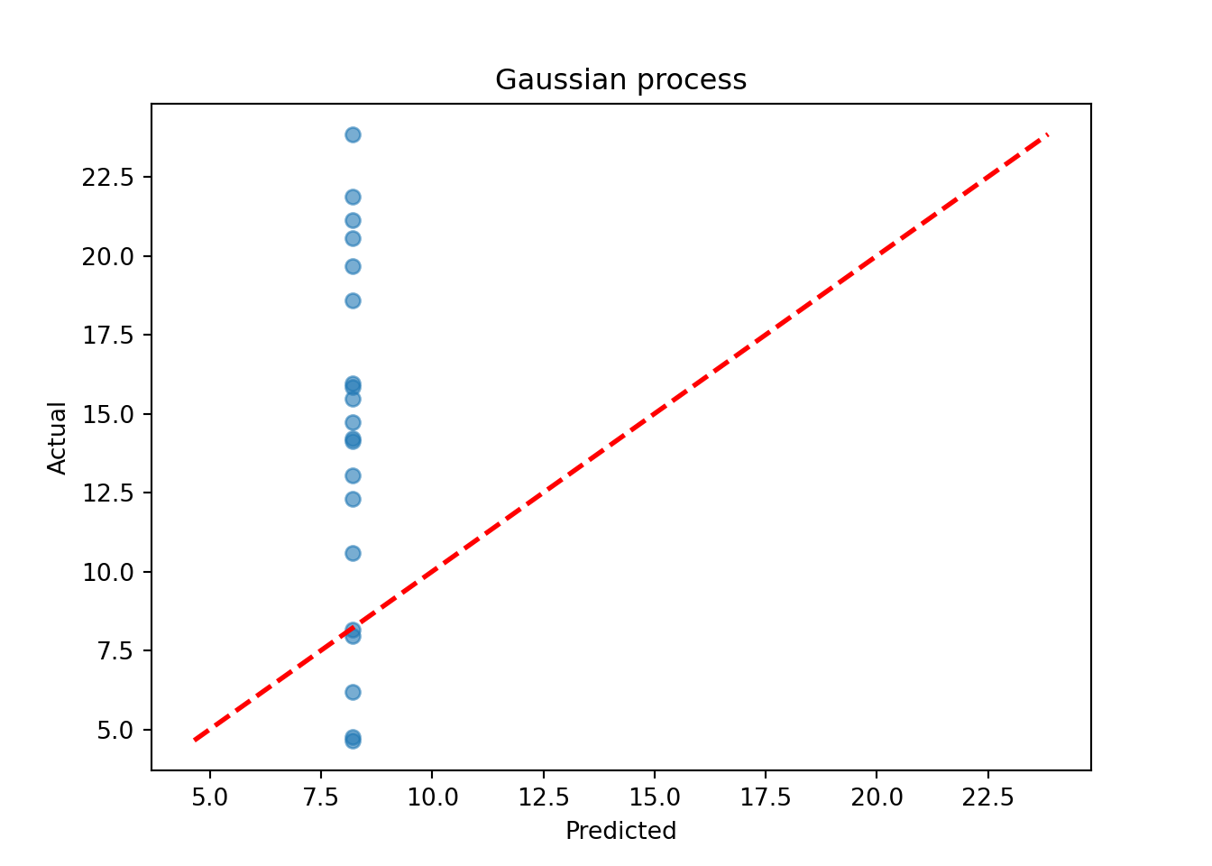

Assess the RMSE

sqrt(mean((model_gp$ZZ.mean - y_test)^2))

[1] 3.39143

print(f"RMSE: {np.sqrt(np.mean((gp_pred_2 - y_test_2)**2)):.4f}")

RMSE: 8.2192

BART-based Gaussian Process

# Run BART on the data
num_trees <- 200
sigma_leaf <- 1/num_trees
X_train <- as.data.frame(X_train)
X_test <- as.data.frame(X_test)
general_params <- list(num_threads=1)
mean_forest_params <- list(num_trees=num_trees, sigma2_leaf_init=sigma_leaf)
bart_model <- bart(X_train=X_train, y_train=y_train, X_test=X_test, 
                   general_params = general_params, mean_forest_params = mean_forest_params)

# Extract kernels needed for kriging
leaf_mat_train <- computeForestLeafIndices(bart_model, X_train, forest_type = "mean",
                                           forest_inds = bart_model$model_params$num_samples - 1)
leaf_mat_test <- computeForestLeafIndices(bart_model, X_test, forest_type = "mean",
                                           forest_inds = bart_model$model_params$num_samples - 1)
W_train <- sparseMatrix(i=rep(1:length(y_train),num_trees), j=leaf_mat_train + 1, x=1)
W_test <- sparseMatrix(i=rep(1:length(y_test),num_trees), j=leaf_mat_test + 1, x=1)
Sigma_11 <- tcrossprod(W_test) / num_trees
Sigma_12 <- tcrossprod(W_test, W_train) / num_trees
Sigma_22 <- tcrossprod(W_train) / num_trees
Sigma_22_inv <- ginv(as.matrix(Sigma_22))
Sigma_21 <- t(Sigma_12)

# Compute mean and covariance for the test set posterior
mu_tilde <- Sigma_12 %*% Sigma_22_inv %*% y_train
Sigma_tilde <- as.matrix((sigma_leaf)*(Sigma_11 - Sigma_12 %*% Sigma_22_inv %*% Sigma_21))

# Sample from f(X_test) | X_test, X_train, f(X_train)
gp_samples <- mvtnorm::rmvnorm(1000, mean = mu_tilde, sigma = Sigma_tilde)

# Compute posterior mean predictions for f(X_test)
yhat_mean_test <- colMeans(gp_samples)
plot(yhat_mean_test, y_test, xlab = "predicted", ylab = "actual", main = "BART Gaussian process")
abline(0,1,lwd=2.5,lty=3,col="red")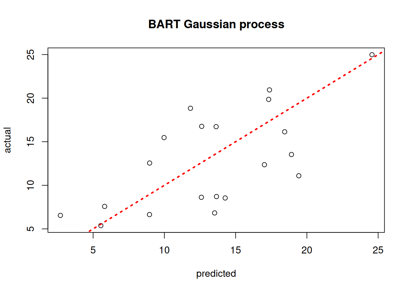

num_trees = 200
sigma_leaf = 1 / num_trees
general_params = {"num_threads": 1}
mean_forest_params = {"num_trees": num_trees, "sigma2_leaf_init": sigma_leaf}
bart_model_2 = BARTModel()
bart_model_2.sample(X_train=X_train_2, y_train=y_train_2, X_test=X_test_2,
                    general_params=general_params, mean_forest_params=mean_forest_params)

last_sample_2 = bart_model_2.num_samples - 1
leaf_mat_train_2 = compute_forest_leaf_indices(bart_model_2, X_train_2,
                                               forest_type="mean", forest_inds=last_sample_2)
leaf_mat_test_2  = compute_forest_leaf_indices(bart_model_2, X_test_2,
                                               forest_type="mean", forest_inds=last_sample_2)

n_train_2, n_test_2 = len(y_train_2), len(y_test_2)
col_inds_train_2 = leaf_mat_train_2.flatten()
col_inds_test_2  = leaf_mat_test_2.flatten()
max_col_2 = max(col_inds_train_2.max(), col_inds_test_2.max()) + 1
W_train_2 = csr_matrix(
    (np.ones(len(col_inds_train_2)),
     (np.tile(np.arange(n_train_2), num_trees), col_inds_train_2)),
    shape=(n_train_2, max_col_2),
)
W_test_2 = csr_matrix(
    (np.ones(len(col_inds_test_2)),
     (np.tile(np.arange(n_test_2), num_trees), col_inds_test_2)),
    shape=(n_test_2, max_col_2),
)

W_tr2 = W_train_2.toarray()
W_te2 = W_test_2.toarray()
Sigma_22_2   = (W_tr2 @ W_tr2.T) / num_trees
Sigma_11_2   = (W_te2 @ W_te2.T) / num_trees
Sigma_12_2   = (W_te2 @ W_tr2.T) / num_trees
Sigma_21_2   = Sigma_12_2.T
Sigma_22_inv_2 = np.linalg.pinv(Sigma_22_2)

mu_tilde_2    = Sigma_12_2 @ Sigma_22_inv_2 @ y_train_2
Sigma_tilde_2 = sigma_leaf * (Sigma_11_2 - Sigma_12_2 @ Sigma_22_inv_2 @ Sigma_21_2)
Sigma_tilde_2 += 1e-8 * np.eye(n_test_2)

gp_samples_2 = rng.multivariate_normal(mu_tilde_2, Sigma_tilde_2, size=1000, method="eigh")
yhat_mean_test_2 = gp_samples_2.mean(axis=0)

lo = min(yhat_mean_test_2.min(), y_test_2.min())
hi = max(yhat_mean_test_2.max(), y_test_2.max())
plt.scatter(yhat_mean_test_2, y_test_2, alpha=0.6)
plt.plot([lo, hi], [lo, hi], color="red", linestyle="dashed", linewidth=2)
plt.xlabel("Predicted")
plt.ylabel("Actual")
plt.title("BART Gaussian process")
plt.show()

Assess the RMSE

sqrt(mean((yhat_mean_test - y_test)^2))

[1] 4.499624

print(f"RMSE: {np.sqrt(np.mean((yhat_mean_test_2 - y_test_2)**2)):.4f}")

RMSE: 3.2809

While the use case of a BART kernel for classical kriging is perhaps unclear without more empirical investigation, the kernel approach can be very beneficial for causal inference applications.

References

Friedman, Jerome H. 1991. “Multivariate Adaptive Regression Splines.” The Annals of Statistics 19 (1): 1–67.

Gramacy, Robert B., and Matthew Taddy. 2010. “Categorical Inputs, Sensitivity Analysis, Optimization and Importance Tempering with tgp Version 2, an R Package for Treed Gaussian Process Models.” Journal of Statistical Software 33 (6): 1–48. https://doi.org/10.18637/jss.v033.i06.

	kernel kernel: kernel instance, default=None The kernel specifying the covariance function of the GP. If None is passed, the kernel ``ConstantKernel(1.0, constant_value_bounds="fixed") * RBF(1.0, length_scale_bounds="fixed")`` is used as default. Note that the kernel hyperparameters are optimized during fitting unless the bounds are marked as "fixed".	RBF(length_sc...se_level=0.01)
	alpha alpha: float or ndarray of shape (n_samples,), default=1e-10 Value added to the diagonal of the kernel matrix during fitting. This can prevent a potential numerical issue during fitting, by ensuring that the calculated values form a positive definite matrix. It can also be interpreted as the variance of additional Gaussian measurement noise on the training observations. Note that this is different from using a `WhiteKernel`. If an array is passed, it must have the same number of entries as the data used for fitting and is used as datapoint-dependent noise level. Allowing to specify the noise level directly as a parameter is mainly for convenience and for consistency with :class:`~sklearn.linear_model.Ridge`. For an example illustrating how the alpha parameter controls the noise variance in Gaussian Process Regression, see :ref:`sphx_glr_auto_examples_gaussian_process_plot_gpr_noisy_targets.py`.	1e-10
	optimizer optimizer: "fmin_l_bfgs_b", callable or None, default="fmin_l_bfgs_b" Can either be one of the internally supported optimizers for optimizing the kernel's parameters, specified by a string, or an externally defined optimizer passed as a callable. If a callable is passed, it must have the signature:: def optimizer(obj_func, initial_theta, bounds): # * 'obj_func': the objective function to be minimized, which # takes the hyperparameters theta as a parameter and an # optional flag eval_gradient, which determines if the # gradient is returned additionally to the function value # * 'initial_theta': the initial value for theta, which can be # used by local optimizers # * 'bounds': the bounds on the values of theta .... # Returned are the best found hyperparameters theta and # the corresponding value of the target function. return theta_opt, func_min Per default, the L-BFGS-B algorithm from `scipy.optimize.minimize` is used. If None is passed, the kernel's parameters are kept fixed. Available internal optimizers are: `{'fmin_l_bfgs_b'}`.	'fmin_l_bfgs_b'
	n_restarts_optimizer n_restarts_optimizer: int, default=0 The number of restarts of the optimizer for finding the kernel's parameters which maximize the log-marginal likelihood. The first run of the optimizer is performed from the kernel's initial parameters, the remaining ones (if any) from thetas sampled log-uniform randomly from the space of allowed theta-values. If greater than 0, all bounds must be finite. Note that `n_restarts_optimizer == 0` implies that one run is performed.	5
	normalize_y normalize_y: bool, default=False Whether or not to normalize the target values `y` by removing the mean and scaling to unit-variance. This is recommended for cases where zero-mean, unit-variance priors are used. Note that, in this implementation, the normalisation is reversed before the GP predictions are reported. .. versionchanged:: 0.23	False
	copy_X_train copy_X_train: bool, default=True If True, a persistent copy of the training data is stored in the object. Otherwise, just a reference to the training data is stored, which might cause predictions to change if the data is modified externally.	True
	n_targets n_targets: int, default=None The number of dimensions of the target values. Used to decide the number of outputs when sampling from the prior distributions (i.e. calling :meth:`sample_y` before :meth:`fit`). This parameter is ignored once :meth:`fit` has been called. .. versionadded:: 1.3	None
	random_state random_state: int, RandomState instance or None, default=None Determines random number generation used to initialize the centers. Pass an int for reproducible results across multiple function calls. See :term:`Glossary `.	101
	kernel__k1	RBF(length_scale=1)
	kernel__k2	WhiteKernel(noise_level=0.01)
	kernel__k1__length_scale	1.0
	kernel__k1__length_scale_bounds	(1e-05, ...)
	kernel__k2__noise_level	0.01
	kernel__k2__noise_level_bounds	(1e-05, ...)

	kernel kernel: kernel instance, default=None The kernel specifying the covariance function of the GP. If None is passed, the kernel ``ConstantKernel(1.0, constant_value_bounds="fixed") * RBF(1.0, length_scale_bounds="fixed")`` is used as default. Note that the kernel hyperparameters are optimized during fitting unless the bounds are marked as "fixed".	RBF(length_sc...noise_level=1)
	alpha alpha: float or ndarray of shape (n_samples,), default=1e-10 Value added to the diagonal of the kernel matrix during fitting. This can prevent a potential numerical issue during fitting, by ensuring that the calculated values form a positive definite matrix. It can also be interpreted as the variance of additional Gaussian measurement noise on the training observations. Note that this is different from using a `WhiteKernel`. If an array is passed, it must have the same number of entries as the data used for fitting and is used as datapoint-dependent noise level. Allowing to specify the noise level directly as a parameter is mainly for convenience and for consistency with :class:`~sklearn.linear_model.Ridge`. For an example illustrating how the alpha parameter controls the noise variance in Gaussian Process Regression, see :ref:`sphx_glr_auto_examples_gaussian_process_plot_gpr_noisy_targets.py`.	1e-10
	optimizer optimizer: "fmin_l_bfgs_b", callable or None, default="fmin_l_bfgs_b" Can either be one of the internally supported optimizers for optimizing the kernel's parameters, specified by a string, or an externally defined optimizer passed as a callable. If a callable is passed, it must have the signature:: def optimizer(obj_func, initial_theta, bounds): # * 'obj_func': the objective function to be minimized, which # takes the hyperparameters theta as a parameter and an # optional flag eval_gradient, which determines if the # gradient is returned additionally to the function value # * 'initial_theta': the initial value for theta, which can be # used by local optimizers # * 'bounds': the bounds on the values of theta .... # Returned are the best found hyperparameters theta and # the corresponding value of the target function. return theta_opt, func_min Per default, the L-BFGS-B algorithm from `scipy.optimize.minimize` is used. If None is passed, the kernel's parameters are kept fixed. Available internal optimizers are: `{'fmin_l_bfgs_b'}`.	'fmin_l_bfgs_b'
	n_restarts_optimizer n_restarts_optimizer: int, default=0 The number of restarts of the optimizer for finding the kernel's parameters which maximize the log-marginal likelihood. The first run of the optimizer is performed from the kernel's initial parameters, the remaining ones (if any) from thetas sampled log-uniform randomly from the space of allowed theta-values. If greater than 0, all bounds must be finite. Note that `n_restarts_optimizer == 0` implies that one run is performed.	1
	normalize_y normalize_y: bool, default=False Whether or not to normalize the target values `y` by removing the mean and scaling to unit-variance. This is recommended for cases where zero-mean, unit-variance priors are used. Note that, in this implementation, the normalisation is reversed before the GP predictions are reported. .. versionchanged:: 0.23	False
	copy_X_train copy_X_train: bool, default=True If True, a persistent copy of the training data is stored in the object. Otherwise, just a reference to the training data is stored, which might cause predictions to change if the data is modified externally.	True
	n_targets n_targets: int, default=None The number of dimensions of the target values. Used to decide the number of outputs when sampling from the prior distributions (i.e. calling :meth:`sample_y` before :meth:`fit`). This parameter is ignored once :meth:`fit` has been called. .. versionadded:: 1.3	None
	random_state random_state: int, RandomState instance or None, default=None Determines random number generation used to initialize the centers. Pass an int for reproducible results across multiple function calls. See :term:`Glossary `.	101
	kernel__k1	RBF(length_scale=1)
	kernel__k2	WhiteKernel(noise_level=1)
	kernel__k1__length_scale	1.0
	kernel__k1__length_scale_bounds	(1e-05, ...)
	kernel__k2__noise_level	1.0
	kernel__k2__noise_level_bounds	(1e-05, ...)