Using Stochtree via Sklearn-Compatible Estimators in Python

This vignette is python-specific and no similar interface is implemented for R.

stochtree.BARTModel is fundamentally a Bayesian interface in which users specify a prior, provide data, sample from the posterior, and manage and inspect the resulting posterior samples. However, the basic BART model

\[y_i \sim \mathcal{N}\left(f(X_i), \sigma^2\right)\]

involves samples of a nonparametric function \(f\) which estimates the expected value of \(y\) given \(X\). Averaging over these draws, the posterior mean \(\bar{f}\) alone may satisfy some supervised learning use cases. To serve this use case straightforwardly, stochtree offers scikit-learn-compatible estimator wrappers around BARTModel which implement the familiar sklearn API.

StochTreeBARTRegressor: continuous outcomes — provides fit, predict, and score
StochTreeBARTBinaryClassifier: binary outcomes via probit BART — provides fit, predict, predict_proba, decision_function, and score
Multi-class classification is supported by wrapping OneVsRestClassifier around StochTreeBARTBinaryClassifier

Setup

import matplotlib.pyplot as plt
import numpy as np
from sklearn.datasets import load_wine, load_breast_cancer
from sklearn.model_selection import GridSearchCV
from sklearn.multiclass import OneVsRestClassifier
from stochtree import (
    StochTreeBARTRegressor,
    StochTreeBARTBinaryClassifier,
)

random_seed = 1234
rng = np.random.default_rng(random_seed)

BART Regression

We simulate simple regression data to demonstrate the continuous outcome case.

n = 100
p = 10
X = rng.normal(size=(n, p))
y = X[:, 0] * 3 + rng.normal(size=n)

We fit a BART regression model by initializing a StochTreeBARTRegressor and calling fit(). Since BARTModel is configured primarily through parameter dictionaries, downstream parameters are passed through as such — here we only specify the random seed.

reg = StochTreeBARTRegressor(general_params={"random_seed": random_seed, "num_threads": 1})
reg.fit(X, y)

StochTreeBARTRegressor(general_params={'num_threads': 1, 'random_seed': 1234})

In a Jupyter environment, please rerun this cell to show the HTML representation or trust the notebook.
On GitHub, the HTML representation is unable to render, please try loading this page with nbviewer.org.

We can then predict from the model and compare posterior mean predictions to the true outcome.

pred = reg.predict(X)
plt.scatter(pred, y)
plt.xlabel("Predicted")
plt.ylabel("Actual")
plt.show()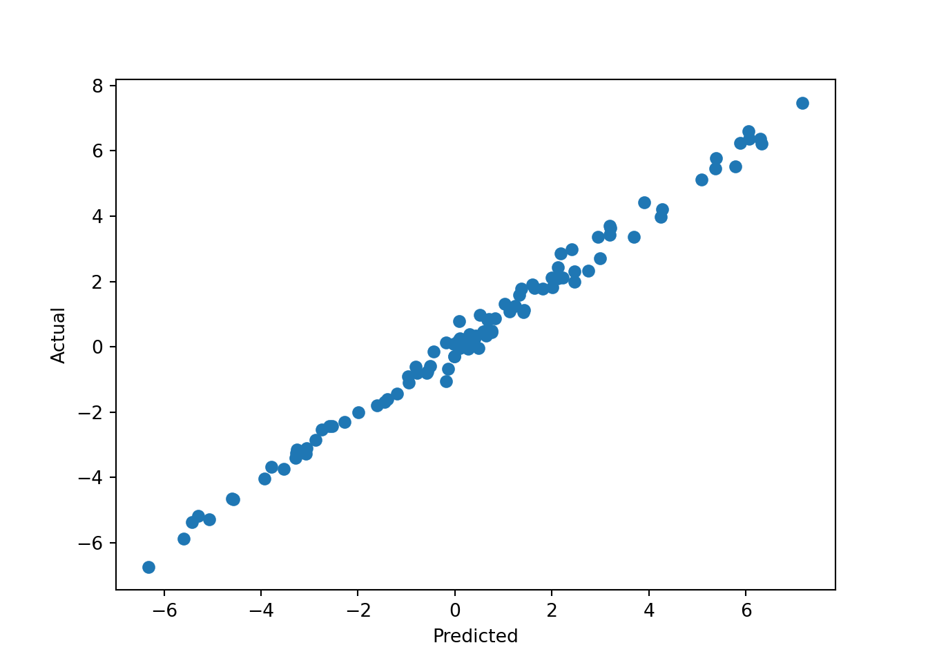

We can also verify determinism by running the model again with the same seed and comparing predictions.

reg2 = StochTreeBARTRegressor(general_params={"random_seed": random_seed, "num_threads": 1})
reg2.fit(X, y)

StochTreeBARTRegressor(general_params={'num_threads': 1, 'random_seed': 1234})

pred2 = reg2.predict(X)
plt.scatter(pred, pred2)
plt.xlabel("First model")
plt.ylabel("Second model")
plt.show()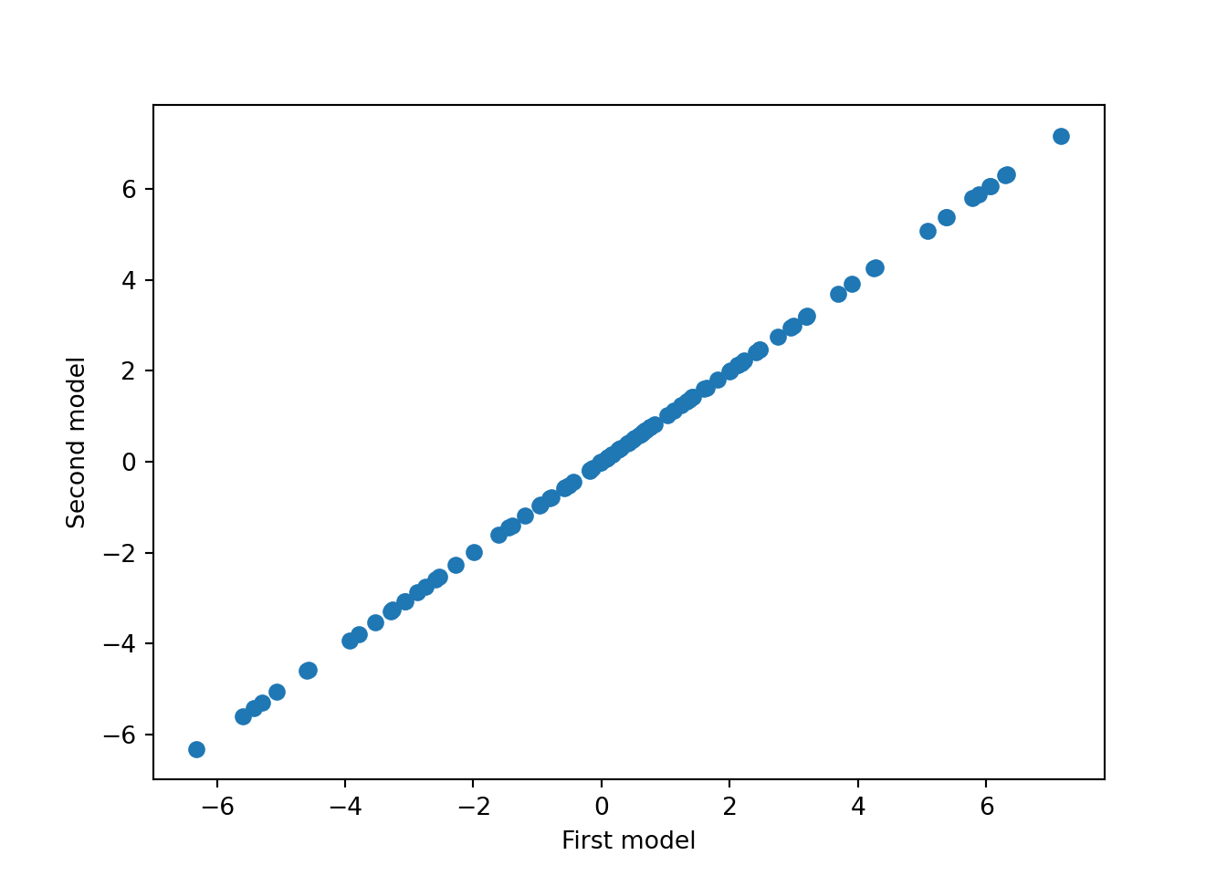

Cross-Validating a BART Model

While the default hyperparameters of BARTModel are designed to work well out of the box, we can use posterior mean prediction error to cross-validate the model’s parameters. Below we use grid search to consider the effect of several BART parameters:

Number of GFR iterations (num_gfr)
Number of MCMC iterations (num_mcmc)
num_trees, alpha, and beta for the mean forest

param_grid = {
    "num_gfr": [10, 40],
    "num_mcmc": [0, 1000],
    "mean_forest_params": [
        {"num_trees": 50, "alpha": 0.95, "beta": 2.0},
        {"num_trees": 100, "alpha": 0.90, "beta": 1.5},
        {"num_trees": 200, "alpha": 0.85, "beta": 1.0},
    ],
}
grid_search = GridSearchCV(
    estimator=StochTreeBARTRegressor(general_params={"num_threads": 1}),
    param_grid=param_grid,
    cv=5,
    scoring="r2",
    n_jobs=1,  # n_jobs=-1 deadlocks when stochtree's C++ thread pool is active
)
grid_search.fit(X, y)

GridSearchCV(cv=5,
             estimator=StochTreeBARTRegressor(general_params={'num_threads': 1}),
             n_jobs=1,
             param_grid={'mean_forest_params': [{'alpha': 0.95, 'beta': 2.0,
                                                 'num_trees': 50},
                                                {'alpha': 0.9, 'beta': 1.5,
                                                 'num_trees': 100},
                                                {'alpha': 0.85, 'beta': 1.0,
                                                 'num_trees': 200}],
                         'num_gfr': [10, 40], 'num_mcmc': [0, 1000]},
             scoring='r2')

Note that we set n_jobs=1 above to avoid deadlocks arising from interactions between reticulate (which renders these python vignettes), joblib, and stochtree’s own C++ multithreading model. Users running this vignette interactively or as a script do not need to fix n_jobs=1.

cv_best_ind = np.argwhere(grid_search.cv_results_['rank_test_score'] == 1).item(0)
best_num_gfr = grid_search.cv_results_['param_num_gfr'][cv_best_ind].item(0)
best_num_mcmc = grid_search.cv_results_['param_num_mcmc'][cv_best_ind].item(0)
best_mean_forest_params = grid_search.cv_results_['param_mean_forest_params'][cv_best_ind]
best_num_trees = best_mean_forest_params['num_trees']
best_alpha = best_mean_forest_params['alpha']
best_beta = best_mean_forest_params['beta']
print_message = f"""
Hyperparameters chosen by grid search:
  num_gfr: {best_num_gfr}
  num_mcmc: {best_num_mcmc}
  num_trees: {best_num_trees}
  alpha: {best_alpha}
  beta: {best_beta}
"""
print(print_message)


Hyperparameters chosen by grid search:
  num_gfr: 40
  num_mcmc: 0
  num_trees: 100
  alpha: 0.9
  beta: 1.5

BART Classification

Binary Classification

We load a binary outcome dataset from sklearn.

dataset = load_breast_cancer()
X = dataset.data
y = dataset.target

We fit a binary classification model using StochTreeBARTBinaryClassifier.

clf = StochTreeBARTBinaryClassifier(general_params={"random_seed": random_seed, "num_threads": 1})
clf.fit(X=X, y=y)

StochTreeBARTBinaryClassifier(general_params={'num_threads': 1,
                                              'random_seed': 1234})

In addition to class predictions, we can compute and visualize the predicted probability of each class via predict_proba().

probs = clf.predict_proba(X)
plt.hist(probs[:, 1], bins=30)
plt.xlabel("Predicted probability (class 1)")
plt.ylabel("Count")
plt.show()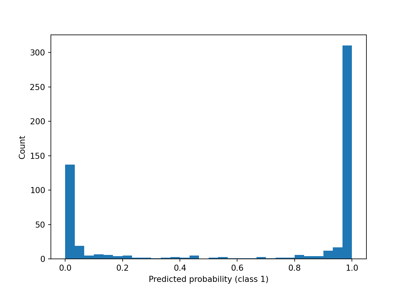

Multi-Class Classification

For multi-class outcomes, we wrap OneVsRestClassifier around StochTreeBARTBinaryClassifier. Here we use the Wine dataset, which has three classes.

dataset = load_wine()
X = dataset.data
y = dataset.target

clf = OneVsRestClassifier(
    StochTreeBARTBinaryClassifier(general_params={"random_seed": random_seed, "num_threads": 1})
)
clf.fit(X=X, y=y)

OneVsRestClassifier(estimator=StochTreeBARTBinaryClassifier(general_params={'num_threads': 1,
                                                                            'random_seed': 1234}))

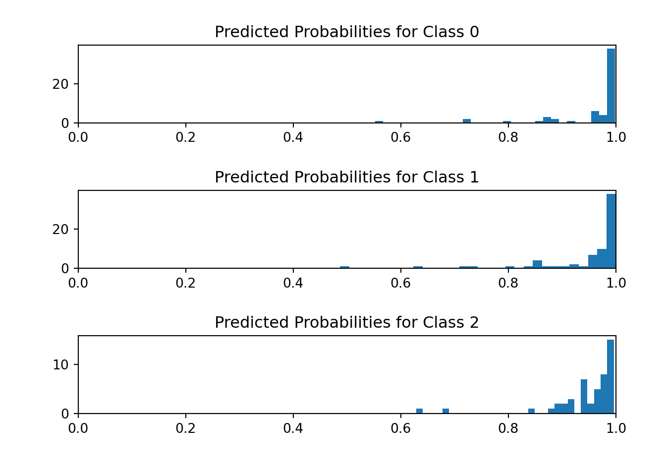
We visualize the histogram of predicted probabilities for each outcome category.

fig, (ax1, ax2, ax3) = plt.subplots(3, 1)
fig.tight_layout(pad=3.0)
probs = clf.predict_proba(X)
ax1.hist(probs[y == 0, 0], bins=30)
ax1.set_title("Predicted Probabilities for Class 0")
ax1.set_xlim(0, 1)

(0.0, 1.0)

ax2.hist(probs[y == 1, 1], bins=30)
ax2.set_title("Predicted Probabilities for Class 1")
ax2.set_xlim(0, 1)

(0.0, 1.0)

ax3.hist(probs[y == 2, 2], bins=30)
ax3.set_title("Predicted Probabilities for Class 2")
ax3.set_xlim(0, 1)

(0.0, 1.0)

plt.show()

	estimator estimator: estimator object This is assumed to implement the scikit-learn estimator interface. Either estimator needs to provide a ``score`` function, or ``scoring`` must be passed.	StochTreeBART..._threads': 1})
	param_grid param_grid: dict or list of dictionaries Dictionary with parameters names (`str`) as keys and lists of parameter settings to try as values, or a list of such dictionaries, in which case the grids spanned by each dictionary in the list are explored. This enables searching over any sequence of parameter settings.	{'mean_forest_params': [{'alpha': 0.95, 'beta': 2.0, 'num_trees': 50}, {'alpha': 0.9, 'beta': 1.5, 'num_trees': 100}, ...], 'num_gfr': [10, 40], 'num_mcmc': [0, 1000]}
	scoring scoring: str, callable, list, tuple or dict, default=None Strategy to evaluate the performance of the cross-validated model on the test set. If `scoring` represents a single score, one can use: - a single string (see :ref:`scoring_string_names`); - a callable (see :ref:`scoring_callable`) that returns a single value; - `None`, the `estimator`'s :ref:`default evaluation criterion ` is used. If `scoring` represents multiple scores, one can use: - a list or tuple of unique strings; - a callable returning a dictionary where the keys are the metric names and the values are the metric scores; - a dictionary with metric names as keys and callables as values. See :ref:`multimetric_grid_search` for an example.	'r2'
	n_jobs n_jobs: int, default=None Number of jobs to run in parallel. ``None`` means 1 unless in a :obj:`joblib.parallel_backend` context. ``-1`` means using all processors. See :term:`Glossary ` for more details. .. versionchanged:: v0.20 `n_jobs` default changed from 1 to None	1
	refit refit: bool, str, or callable, default=True Refit an estimator using the best found parameters on the whole dataset. For multiple metric evaluation, this needs to be a `str` denoting the scorer that would be used to find the best parameters for refitting the estimator at the end. Where there are considerations other than maximum score in choosing a best estimator, ``refit`` can be set to a function which returns the selected ``best_index_`` given ``cv_results_``. In that case, the ``best_estimator_`` and ``best_params_`` will be set according to the returned ``best_index_`` while the ``best_score_`` attribute will not be available. The refitted estimator is made available at the ``best_estimator_`` attribute and permits using ``predict`` directly on this ``GridSearchCV`` instance. Also for multiple metric evaluation, the attributes ``best_index_``, ``best_score_`` and ``best_params_`` will only be available if ``refit`` is set and all of them will be determined w.r.t this specific scorer. See ``scoring`` parameter to know more about multiple metric evaluation. See :ref:`sphx_glr_auto_examples_model_selection_plot_grid_search_digits.py` to see how to design a custom selection strategy using a callable via `refit`. See :ref:`this example ` for an example of how to use ``refit=callable`` to balance model complexity and cross-validated score. .. versionchanged:: 0.20 Support for callable added.	True
	cv cv: int, cross-validation generator or an iterable, default=None Determines the cross-validation splitting strategy. Possible inputs for cv are: - None, to use the default 5-fold cross validation, - integer, to specify the number of folds in a `(Stratified)KFold`, - :term:`CV splitter`, - An iterable yielding (train, test) splits as arrays of indices. For integer/None inputs, if the estimator is a classifier and ``y`` is either binary or multiclass, :class:`StratifiedKFold` is used. In all other cases, :class:`KFold` is used. These splitters are instantiated with `shuffle=False` so the splits will be the same across calls. Refer :ref:`User Guide ` for the various cross-validation strategies that can be used here. .. versionchanged:: 0.22 ``cv`` default value if None changed from 3-fold to 5-fold.	5
	verbose verbose: int Controls the verbosity: the higher, the more messages. - >1 : the computation time for each fold and parameter candidate is displayed; - >2 : the score is also displayed; - >3 : the fold and candidate parameter indexes are also displayed together with the starting time of the computation.	0
	pre_dispatch pre_dispatch: int, or str, default='2n_jobs' Controls the number of jobs that get dispatched during parallel execution. Reducing this number can be useful to avoid an explosion of memory consumption when more jobs get dispatched than CPUs can process. This parameter can be: - None, in which case all the jobs are immediately created and spawned. Use this for lightweight and fast-running jobs, to avoid delays due to on-demand spawning of the jobs - An int, giving the exact number of total jobs that are spawned - A str, giving an expression as a function of n_jobs, as in '2n_jobs'	'2*n_jobs'
	error_score error_score: 'raise' or numeric, default=np.nan Value to assign to the score if an error occurs in estimator fitting. If set to 'raise', the error is raised. If a numeric value is given, FitFailedWarning is raised. This parameter does not affect the refit step, which will always raise the error.	nan
	return_train_score return_train_score: bool, default=False If ``False``, the ``cv_results_`` attribute will not include training scores. Computing training scores is used to get insights on how different parameter settings impact the overfitting/underfitting trade-off. However computing the scores on the training set can be computationally expensive and is not strictly required to select the parameters that yield the best generalization performance. .. versionadded:: 0.19 .. versionchanged:: 0.21 Default value was changed from ``True`` to ``False``	False

	estimator estimator: estimator object A regressor or a classifier that implements :term:`fit`. When a classifier is passed, :term:`decision_function` will be used in priority and it will fallback to :term:`predict_proba` if it is not available. When a regressor is passed, :term:`predict` is used.	StochTreeBART..._seed': 1234})
	n_jobs n_jobs: int, default=None The number of jobs to use for the computation: the `n_classes` one-vs-rest problems are computed in parallel. ``None`` means 1 unless in a :obj:`joblib.parallel_backend` context. ``-1`` means using all processors. See :term:`Glossary ` for more details. .. versionchanged:: 0.20 `n_jobs` default changed from 1 to None	None
	verbose verbose: int, default=0 The verbosity level, if non zero, progress messages are printed. Below 50, the output is sent to stderr. Otherwise, the output is sent to stdout. The frequency of the messages increases with the verbosity level, reporting all iterations at 10. See :class:`joblib.Parallel` for more details. .. versionadded:: 1.1	0

	num_gfr	10
	num_burnin	0
	num_mcmc	100
	general_params	{'num_threads': 1, 'random_seed': 1234}
	mean_forest_params	None
	variance_forest_params	None
	rfx_params	None

	num_gfr	10
	num_burnin	0
	num_mcmc	100
	general_params	{'num_threads': 1, 'random_seed': 1234}
	mean_forest_params	None
	variance_forest_params	None
	rfx_params	None

	num_gfr	40
	num_burnin	0
	num_mcmc	0
	general_params	{'num_threads': 1}
	mean_forest_params	{'alpha': 0.9, 'beta': 1.5, 'num_trees': 100}
	variance_forest_params	None
	rfx_params	None

	num_gfr	10
	num_burnin	0
	num_mcmc	100
	general_params	{'num_threads': 1, 'random_seed': 1234}
	mean_forest_params	None
	variance_forest_params	None
	rfx_params	None