Regression Discontinuity Design (RDD) with StochTree

Introduction

We study conditional average treatment effect (CATE) estimation for regression discontinuity designs (RDD), in which treatment assignment is based on whether a particular covariate — referred to as the running variable — lies above or below a known value, referred to as the cutoff value. Because treatment is deterministically assigned as a known function of the running variable, RDDs are trivially deconfounded: treatment assignment is independent of the outcome variable, given the running variable. However, estimation of treatment effects in RDDs is more complicated than simply controlling for the running variable, because doing so introduces a complete lack of overlap. Nonetheless, the CATE at the cutoff, \(X=c\), may still be identified provided the conditional expectation \(E[Y \mid X,W]\) is continuous at that point for all \(W=w\). We exploit this assumption with the leaf regression BART model implemented in stochtree, which allows us to define an explicit prior on the CATE.

Regression Discontinuity Design

We conceptualize the treatment effect estimation problem via a quartet of random variables \((Y, X, Z, U)\). The variable \(Y\) is the outcome variable; \(X\) is the running variable; \(Z\) is the treatment assignment indicator; and \(U\) represents additional, possibly unobserved, causal factors. What makes this an RDD is the stipulation that \(Z = I(X > c)\) for cutoff \(c\). We assume \(c = 0\) without loss of generality.

The following figure depicts a causal diagram representing the assumed causal relationships between these variables. Two key features are: (1) \(X\) blocks the impact of \(U\) on \(Z\), satisfying the back-door criterion; and (2) \(X\) and \(U\) are not descendants of \(Z\).

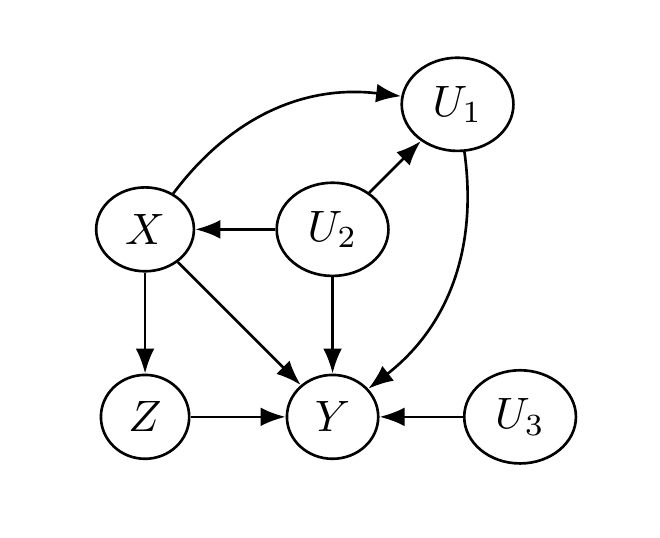
A causal directed acyclic graph representing the general structure of a regression discontinuity design problem.

Using this causal diagram, we may express \(Y\) as some function of its graph parents \((X,Z,U)\): \(Y = \F(X,Z,U)\). We relate this to the potential outcomes framework via

\[ Y^1 = \F(X,1,U), \qquad Y^0 = \F(X,0,U). \]

Defining conditional expectations \[ \mu_1(x) = E[Y \mid X=x, Z=1], \qquad \mu_0(x) = E[Y \mid X=x, Z=0], \] the treatment effect function is \(\tau(x) = \mu_1(x) - \mu_0(x)\). Because \(Z = I(X > 0)\), we can only learn \(\mu_1(x)\) for \(X > 0\) and \(\mu_0(x)\) for \(X < 0\). Overlap is violated, so the overall ATE \(\bar{\tau} = E(\tau(X))\) is unidentified. We instead estimate \(\tau(0) = \mu_1(0) - \mu_0(0)\), which is identified for continuous \(X\) under the assumption that \(\mu_1\) and \(\mu_0\) are suitably smooth at \(x = 0\).

Conditional Average Treatment Effects in RDD

We are concerned with learning not only \(\tau(0)\) but also RDD CATEs, \(\tau(0, \w)\) for covariate vector \(\w\). Defining potential outcome means

\[ \mu_z(x,\w) = E[Y \mid X=x, W=\w, Z=z], \]

our treatment effect function is \(\tau(x,\w) = \mu_1(x,\w) - \mu_0(x,\w)\). We must assume \(\mu_1(x,\w)\) and \(\mu_0(x,\w)\) are suitably smooth in \(x\) for every \(\w\). CATE estimation in RDDs then reduces to estimating \(E[Y \mid X=x, W=\w, Z=z]\), for which we turn to BART.

The BARDDT Model

We propose a BART model where the trees split on \((x,\w)\) but each leaf node parameter is a vector of regression coefficients tailored to the RDD context. Let \(\psi\) denote the following basis vector: \[ \psi(x,z) = \begin{bmatrix} 1 & zx & (1-z)x & z \end{bmatrix}. \]

The prediction function for tree \(j\) is defined as \(g_j(x, \w, z) = \psi(x, z) \Gamma_{b_j(x, \w)}\) for leaf-specific regression vector \(\Gamma_{b_j} = (\eta_{b_j}, \lambda_{b_j}, \theta_{b_j}, \Delta_{b_j})^t\). The model for observations in leaf \(b_j\) is

\[ \Y_{b_j} \mid \Gamma_{b_j}, \sigma^2 \sim \N(\Psi_{b_j} \Gamma_{b_j}, \sigma^2), \qquad \Gamma_{b_j} \sim \N(0, \Sigma_0), \]

where we set \(\Sigma_0 = \frac{0.033}{J}\mathrm{I}\) as a default (for \(x\) standardized to unit variance in-sample).

This choice of basis entails that the RDD CATE at \(\w\), \(\tau(0, \w)\), is the sum of the \(\Delta_{b_j(0, \w)}\) elements across all trees:

\[ \tau(0, \w) = \sum_{j=1}^J \Delta_{b_j(0, \w)}. \]

The priors on the \(\Delta\) coefficients directly regularize the treatment effect.

The following figures illustrate how BARDDT fits a response surface and estimates CATEs.

Two regression trees with splits in \(x\) and a single scalar \(w\). Node images depict the \(g(x,w,z)\) function defined by that node’s coefficients. The vertical gap between line segments at \(x=0\) is that node’s contribution to the CATE.

The same two trees represented as a partition of the \(x\)-\(w\) plane. The bottom figure shows the combined partition; the red dashed line marks \(W=w^*\).

Left: the function fit at \(W = w^*\) for the two trees, superimposed. Right: the aggregated fit. The magnitude of the discontinuity at \(x = 0\) is the treatment effect.

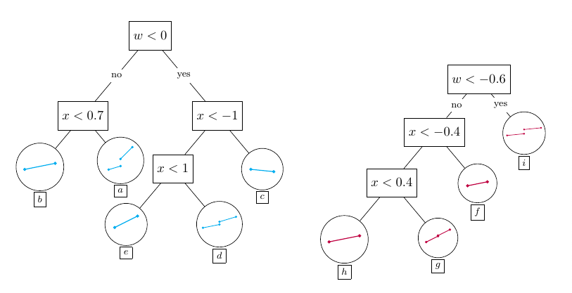
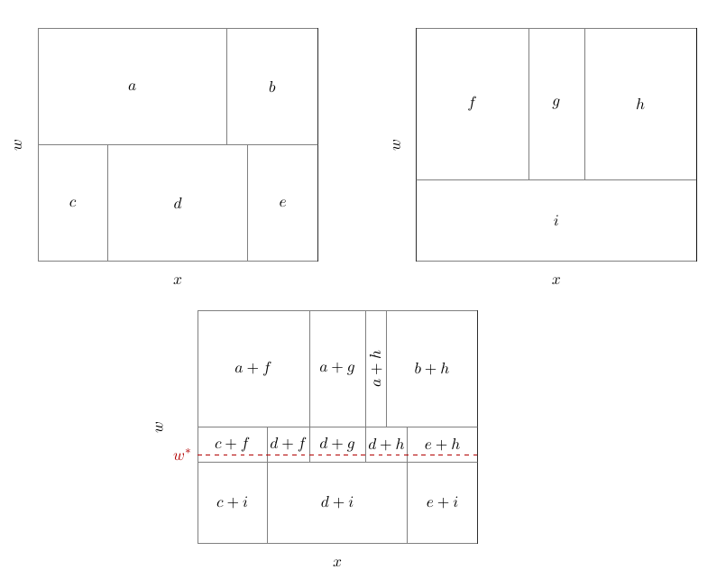
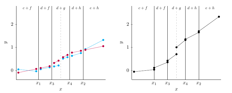
An interesting property of BARDDT: by letting the regression trees split on the running variable, there is no need to separately define a bandwidth as in polynomial RDD. The regression trees automatically determine (in the course of posterior sampling) when to prune away regions far from the cutoff.

Demo

In this section, we provide code for implementing BARDDT in stochtree on a popular RDD dataset.

Setup

Load the necessary packages

library(stochtree)
library(rpart)
library(rpart.plot)
library(foreach)
library(doParallel)

import matplotlib.pyplot as plt
import seaborn as sns
import numpy as np
import pandas as pd
from sklearn.tree import DecisionTreeRegressor, plot_tree
from stochtree import BARTModel

Set a seed for reproducibility

random_seed <- 1234
set.seed(random_seed)

random_seed = 1234
rng = np.random.default_rng(random_seed)

Dataset

The data comes from Lindo et al. (2010), who analyze data on college students at a large Canadian university to evaluate an academic probation policy. Students whose GPA falls below a threshold are placed on academic probation. The running variable \(X\) is the negative distance between a student’s previous-term GPA and the probation threshold, so students on probation (\(Z = 1\)) have positive scores and the cutoff is 0. The outcome \(Y\) is the student’s GPA at the end of the current term. Potential moderators \(W\) are: gender (male), age at university entry (age_at_entry), a dummy for being born in North America (bpl_north_america), credits taken in the first year (totcredits_year1), campus indicators (loc_campus 1–3), and high school GPA quantile (hsgrade_pct).

# Load and organize data
data <- read.csv("https://raw.githubusercontent.com/rdpackages-replication/CIT_2024_CUP/refs/heads/main/CIT_2024_CUP_discrete.csv")
y <- data$nextGPA
x <- data$X
n <- nrow(data)

# Standardize x
x <- x / sd(x)

# Extract covariates
w <- data[, 4:11]

# Encode categorical features as ordered/unordered factors
w$totcredits_year1 <- factor(w$totcredits_year1, ordered = TRUE)
w$male <- factor(w$male, ordered = FALSE)
w$bpl_north_america <- factor(w$bpl_north_america, ordered = FALSE)
w$loc_campus1 <- factor(w$loc_campus1, ordered = FALSE)
w$loc_campus2 <- factor(w$loc_campus2, ordered = FALSE)
w$loc_campus3 <- factor(w$loc_campus3, ordered = FALSE)

# x is normalized so the cutoff occurs at c = 0
c <- 0

# Binarize the running variable into a "treatment" indicator
z <- as.numeric(x > c)

# Window for prediction sample
h <- 0.1

# Define the prediction subset
test <- -h < x & x < h
ntest <- sum(test)

# Load and organize data
data = pd.read_csv("https://raw.githubusercontent.com/rdpackages-replication/CIT_2024_CUP/refs/heads/main/CIT_2024_CUP_discrete.csv")
y = data.loc[:, "nextGPA"].to_numpy().squeeze()
x = data.loc[:, "X"].to_numpy().squeeze()
n = data.shape[0]

# Standardize x
x = x / np.std(x)

# Extract covariates
w = data.iloc[:, 3:11]

# Encode categorical features as ordered/unordered factors
w["totcredits_year1"] = pd.Categorical(
    w["totcredits_year1"], ordered=True
)
unordered_categorical_cols = [
    "male",
    "bpl_north_america",
    "loc_campus1",
    "loc_campus2",
    "loc_campus3",
]
for col in unordered_categorical_cols:
    w.loc[:, col] = pd.Categorical(w.loc[:, col], ordered=False)

# x is normalized so the cutoff occurs at c = 0
c = 0

# Binarize the running variable into a "treatment" indicator
z = (x > c).astype(float)

# Window for prediction sample
h = 0.1

# Define the prediction subset
test = (-h < x) & (x < h)
ntest = np.sum(test)

Target Estimand

Our estimand is the CATE function at \(x = 0\), i.e. \(\tau(0, \w)\). To focus on feasible estimation points, we restrict to observed \(\w_i\) such that \(|x_i| \leq \delta\) (here \(\delta = 0.1\) after standardizing \(X\)). Our estimand is therefore

\[ \tau(0, \w_i) \quad \forall i \text{ such that } |x_i| \leq \delta. \]

Implementing BARDDT

The \(\psi\) basis vector for the leaf regression is \(\psi = [1,\, zx,\, (1-z)x,\, z]\), and the training covariate matrix is \([x,\, W]\). The prediction basis at the cutoff for \(Z=1\) and \(Z=0\) is

\[ \psi_1 = [1, 0, 0, 1], \qquad \psi_0 = [1, 0, 0, 0]. \]

Psi <- cbind(rep(1, n), z * x, (1 - z) * x, z)

Psi = np.c_[np.ones(n), z * x, (1 - z) * x, z]

Fitting the Model

We run multiple chains and combine their posterior draws. To compute the CATE posterior, we obtain \(Y(z)\) predictions by predicting from the model with \(Z = z\) set in the basis. stochtree provides a function / method (computeContrastBARTModel in R, compute_contrast in Python) for directly computing this contrast from a sampled BART model.

# Define sampling parameters
num_chains <- 4
num_gfr <- 4
num_burnin <- 0
num_mcmc <- 500

# Parameter lists for BART model fit
global_params <- list(
  standardize = T,
  sample_sigma_global = TRUE,
  sigma2_global_init = 0.1, 
  random_seed = random_seed, 
  num_threads = 1, 
  num_chains = num_chains
)
forest_params <- list(
  num_trees = 50,
  min_samples_leaf = 20,
  alpha = 0.95,
  beta = 2,
  max_depth = 20,
  sample_sigma2_leaf = FALSE,
  sigma2_leaf_init = 0.1 / 50
)

# Fit the BART model
bart_model <- bart(
  X_train = cbind(x, w),
  leaf_basis_train = Psi,
  y_train = y,
  num_gfr = num_gfr,
  num_burnin = num_burnin,
  num_mcmc = num_mcmc,
  general_params = global_params,
  mean_forest_params = forest_params
)

# Compute the CATE posterior
Psi0 <- cbind(rep(1, n), rep(0, n), rep(0, n), rep(0, n))[test, ]
Psi1 <- cbind(rep(1, n), rep(0, n), rep(0, n), rep(1, n))[test, ]
covariates_test <- cbind(x = rep(0, n), w)[test, ]
cate_posterior <- computeContrastBARTModel(
  bart_model,
  X_0 = covariates_test,
  X_1 = covariates_test,
  leaf_basis_0 = Psi0,
  leaf_basis_1 = Psi1,
  type = "posterior",
  scale = "linear"
)

# Define sampling parameters
num_chains = 4
num_gfr = 4
num_burnin = 0
num_mcmc = 500

# Parameter lists for BART model fit
global_params = {
    "standardize": True,
    "sample_sigma_global": True,
    "sigma2_global_init": 0.1,
    "random_seed": random_seed,
    "num_threads": 1, 
    "num_chains": num_chains
}
forest_params = {
    "num_trees": 50,
    "min_samples_leaf": 20,
    "alpha": 0.95,
    "beta": 2,
    "max_depth": 20,
    "sample_sigma2_leaf": False,
    "sigma2_leaf_init": 0.1 / 50,
}

# Fit the BART model
covariates_train = w
covariates_train.loc[:, "x"] = x
bart_model = BARTModel()
bart_model.sample(
    X_train=covariates_train,
    leaf_basis_train=Psi,
    y_train=y,
    num_gfr=num_gfr,
    num_burnin=num_burnin,
    num_mcmc=num_mcmc,
    general_params=global_params,
    mean_forest_params=forest_params,
)

# Compute the CATE posterior
Psi0 = np.c_[np.ones(n), np.zeros(n), np.zeros(n), np.zeros(n)][test, :]
Psi1 = np.c_[np.ones(n), np.zeros(n), np.zeros(n), np.ones(n)][test, :]
covariates_test = w.iloc[test, :]
covariates_test.loc[:, "x"] = np.zeros(ntest)
cate_posterior = bart_model.compute_contrast(
    X_0=covariates_test,
    X_1=covariates_test,
    leaf_basis_0=Psi0,
    leaf_basis_1=Psi1,
    type="posterior",
    scale="linear",
)

Analyzing CATE Heterogeneity

To summarize the CATE posterior we fit a regression tree to the posterior mean point estimates \(\bar{\tau}_i = \frac{1}{M} \sum_{h=1}^M \tau^{(h)}(0, \w_i)\), using \(W\) as predictors. We restrict to observations with \(|x_i| \leq \delta\).

cate <- rpart(y ~ ., data.frame(y = rowMeans(cate_posterior), w[test, ]),
              control = rpart.control(cp = 0.015))

plot_cart <- function(rp) {
  fr    <- rp$frame
  left  <- which.min(fr$yval)
  right <- which.max(fr$yval)
  cols  <- rep("lightblue3", nrow(fr))
  cols[fr$yval == fr$yval[left]]  <- "tomato3"
  cols[fr$yval == fr$yval[right]] <- "gold2"
  cols
}

rpart.plot(cate, main = "", box.col = plot_cart(cate))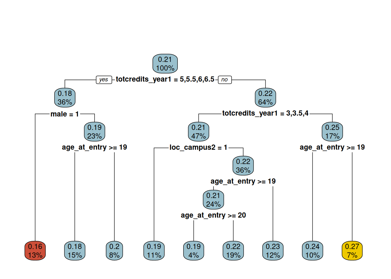

Regression tree fit to posterior point estimates of individual treatment effects. Top number in each box is the average subgroup treatment effect; lower number is the share of the sample.

y_surrogate  = np.mean(cate_posterior, axis=1)
X_surrogate  = w.iloc[test, :]
cp = 0.015
min_impurity_decrease = cp * np.var(y_surrogate)
cate_tree = DecisionTreeRegressor(min_impurity_decrease=min_impurity_decrease)
cate_tree.fit(X=X_surrogate, y=y_surrogate)

DecisionTreeRegressor(min_impurity_decrease=np.float64(2.1112270825828327e-05))

In a Jupyter environment, please rerun this cell to show the HTML representation or trust the notebook.
On GitHub, the HTML representation is unable to render, please try loading this page with nbviewer.org.

Decision tree fit to posterior mean CATEs, used as an effect moderation summary.

plot_tree(cate_tree, impurity=False, filled=True,
          feature_names=w.columns, proportion=False,
          label="root", node_ids=True)
plt.show()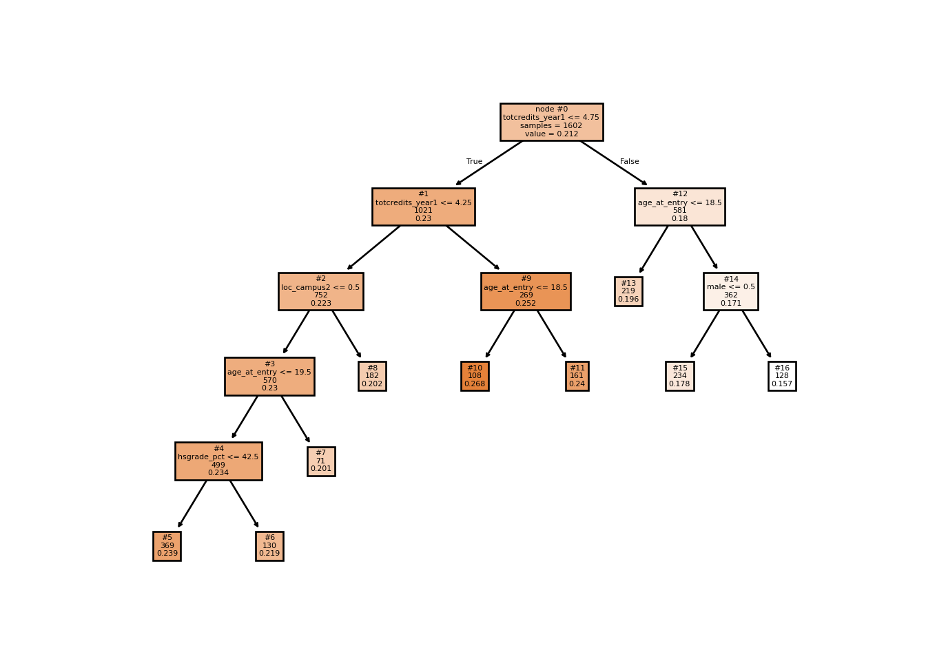

The resulting tree indicates that course load (totcredits_year1) in the academic term leading to probation is a strong moderator of the treatment effect. The tree also flags campus, age at entry, and gender as secondary moderators — all prima facie plausible.

Comparing Subgroup Posteriors

The effect moderation tree is a posterior summary tool; it does not alter the posterior itself. We can compare any two subgroups by averaging their individual posterior draws. Consider the two groups at opposite ends of the effect range:

Group A: male student, entered college older than 19, attempted > 4.8 credits in the first year (leftmost leaf, red)
Group B: any gender, entered college younger than 19, attempted 4.3–4.8 credits in the first year (rightmost leaf, gold)

Subgroup posteriors are

\[ \bar{\tau}_A^{(h)} = \frac{1}{n_A} \sum_{i \in A} \tau^{(h)}(0, \w_i), \]

where \(h\) indexes a posterior draw and \(n_A\) is the group size.

cate_kde <- function(rp, pred) {
  left   <- rp$where == which.min(rp$frame$yval)
  right  <- rp$where == which.max(rp$frame$yval)
  cate_a <- colMeans(pred[left,  , drop = FALSE])
  cate_b <- colMeans(pred[right, , drop = FALSE])
  MASS::kde2d(cate_a, cate_b, n = 200)
}
contour(cate_kde(cate, cate_posterior), bty = "n",
        xlab = "Group A", ylab = "Group B")
abline(a = 0, b = 1)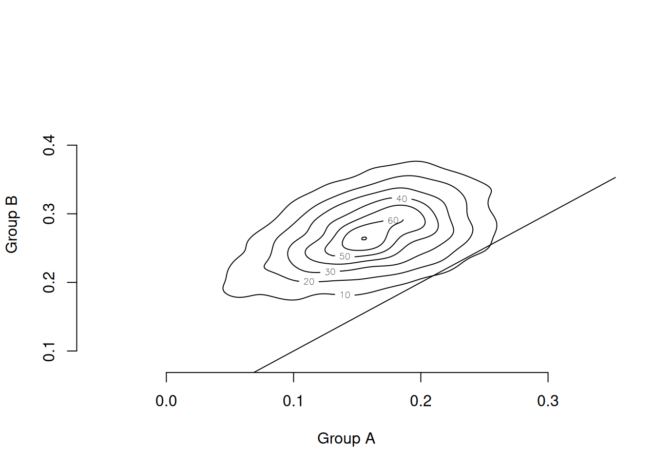

Joint kernel density estimate of the CATE posteriors for Groups A and B. Nearly all contour lines lie above the 45° line, indicating that Group B has persistently higher treatment effects.

predicted_nodes  = cate_tree.apply(X=X_surrogate)
max_value_node = np.argmax(cate_tree.tree_.value)
min_value_node = np.argmin(cate_tree.tree_.value)
posterior_group_a = np.mean(cate_posterior[predicted_nodes == min_value_node, :], axis=0)
posterior_group_b = np.mean(cate_posterior[predicted_nodes == max_value_node, :], axis=0)
posterior_df = pd.DataFrame({"group_a": posterior_group_a,
                             "group_b": posterior_group_b})
sns.kdeplot(data=posterior_df, x="group_a", y="group_b")
plt.axline((0, 0), slope=1, color="black", linestyle=(0, (3, 3)))
plt.show()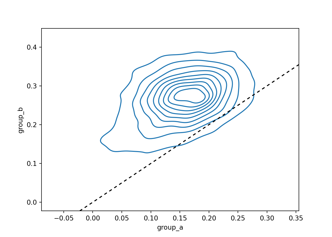

Joint KDE of Group A and Group B CATE posteriors. Contours above the diagonal indicate Group B has persistently higher treatment effects.

The contour lines are nearly all above the 45° line, indicating that the posterior probability mass lies in the region where Group B has a larger treatment effect than Group A, even after accounting for estimation uncertainty.

As always, CATEs that vary with observable factors do not necessarily represent a causal moderating relationship; uncovering these patterns is crucial for suggesting causal mechanisms to investigate in future studies.

References

Lindo, Jason M, Nicholas J Sanders, and Philip Oreopoulos. 2010. “Ability, Gender, and Performance Standards: Evidence from Academic Probation.” American Economic Journal: Applied Economics 2 (2): 95–117.

	criterion criterion: {"squared_error", "friedman_mse", "absolute_error", "poisson"}, default="squared_error" The function to measure the quality of a split. Supported criteria are "squared_error" for the mean squared error, which is equal to variance reduction as feature selection criterion and minimizes the L2 loss using the mean of each terminal node, "friedman_mse", which uses mean squared error with Friedman's improvement score for potential splits, "absolute_error" for the mean absolute error, which minimizes the L1 loss using the median of each terminal node, and "poisson" which uses reduction in the half mean Poisson deviance to find splits. .. versionadded:: 0.18 Mean Absolute Error (MAE) criterion. .. versionadded:: 0.24 Poisson deviance criterion.	'squared_error'
	splitter splitter: {"best", "random"}, default="best" The strategy used to choose the split at each node. Supported strategies are "best" to choose the best split and "random" to choose the best random split.	'best'
	max_depth max_depth: int, default=None The maximum depth of the tree. If None, then nodes are expanded until all leaves are pure or until all leaves contain less than min_samples_split samples. For an example of how ``max_depth`` influences the model, see :ref:`sphx_glr_auto_examples_tree_plot_tree_regression.py`.	None
	min_samples_split min_samples_split: int or float, default=2 The minimum number of samples required to split an internal node: - If int, then consider `min_samples_split` as the minimum number. - If float, then `min_samples_split` is a fraction and `ceil(min_samples_split * n_samples)` are the minimum number of samples for each split. .. versionchanged:: 0.18 Added float values for fractions.	2
	min_samples_leaf min_samples_leaf: int or float, default=1 The minimum number of samples required to be at a leaf node. A split point at any depth will only be considered if it leaves at least ``min_samples_leaf`` training samples in each of the left and right branches. This may have the effect of smoothing the model, especially in regression. - If int, then consider `min_samples_leaf` as the minimum number. - If float, then `min_samples_leaf` is a fraction and `ceil(min_samples_leaf * n_samples)` are the minimum number of samples for each node. .. versionchanged:: 0.18 Added float values for fractions.	1
	min_weight_fraction_leaf min_weight_fraction_leaf: float, default=0.0 The minimum weighted fraction of the sum total of weights (of all the input samples) required to be at a leaf node. Samples have equal weight when sample_weight is not provided.	0.0
	max_features max_features: int, float or {"sqrt", "log2"}, default=None The number of features to consider when looking for the best split: - If int, then consider `max_features` features at each split. - If float, then `max_features` is a fraction and `max(1, int(max_features * n_features_in_))` features are considered at each split. - If "sqrt", then `max_features=sqrt(n_features)`. - If "log2", then `max_features=log2(n_features)`. - If None, then `max_features=n_features`. Note: the search for a split does not stop until at least one valid partition of the node samples is found, even if it requires to effectively inspect more than ``max_features`` features.	None
	random_state random_state: int, RandomState instance or None, default=None Controls the randomness of the estimator. The features are always randomly permuted at each split, even if ``splitter`` is set to ``"best"``. When ``max_features < n_features``, the algorithm will select ``max_features`` at random at each split before finding the best split among them. But the best found split may vary across different runs, even if ``max_features=n_features``. That is the case, if the improvement of the criterion is identical for several splits and one split has to be selected at random. To obtain a deterministic behaviour during fitting, ``random_state`` has to be fixed to an integer. See :term:`Glossary ` for details.	None
	max_leaf_nodes max_leaf_nodes: int, default=None Grow a tree with ``max_leaf_nodes`` in best-first fashion. Best nodes are defined as relative reduction in impurity. If None then unlimited number of leaf nodes.	None
	min_impurity_decrease min_impurity_decrease: float, default=0.0 A node will be split if this split induces a decrease of the impurity greater than or equal to this value. The weighted impurity decrease equation is the following:: N_t / N * (impurity - N_t_R / N_t * right_impurity - N_t_L / N_t * left_impurity) where ``N`` is the total number of samples, ``N_t`` is the number of samples at the current node, ``N_t_L`` is the number of samples in the left child, and ``N_t_R`` is the number of samples in the right child. ``N``, ``N_t``, ``N_t_R`` and ``N_t_L`` all refer to the weighted sum, if ``sample_weight`` is passed. .. versionadded:: 0.19	np.float64(2....825828327e-05)
	ccp_alpha ccp_alpha: non-negative float, default=0.0 Complexity parameter used for Minimal Cost-Complexity Pruning. The subtree with the largest cost complexity that is smaller than ``ccp_alpha`` will be chosen. By default, no pruning is performed. See :ref:`minimal_cost_complexity_pruning` for details. See :ref:`sphx_glr_auto_examples_tree_plot_cost_complexity_pruning.py` for an example of such pruning. .. versionadded:: 0.22	0.0
	monotonic_cst monotonic_cst: array-like of int of shape (n_features), default=None Indicates the monotonicity constraint to enforce on each feature. - 1: monotonic increase - 0: no constraint - -1: monotonic decrease If monotonic_cst is None, no constraints are applied. Monotonicity constraints are not supported for: - multioutput regressions (i.e. when `n_outputs_ > 1`), - regressions trained on data with missing values. Read more in the :ref:`User Guide `. .. versionadded:: 1.4	None