Examining Individual Trees in a Fitted Ensemble

While out of sample evaluation and MCMC diagnostics on parametric BART components (i.e. \(\sigma^2\), the global error variance) are helpful, it’s important to be able to inspect the trees in a BART / BCF model. This vignette walks through some of the features stochtree provides to query and understand the forests and trees in a model.

Setup

Load necessary packages

R

library(stochtree)

Python

import numpy as np
import matplotlib.pyplot as plt
from stochtree import BARTModel

Set a seed for reproducibility

R

random_seed = 1234
set.seed(random_seed)

Python

random_seed = 1234
rng = np.random.default_rng(random_seed)

Data Generation

Generate sample data where feature 10 is the only “important” feature

R

n <- 500
p_x <- 10
X <- matrix(runif(n*p_x), ncol = p_x)
f_XW <- (
    ((0 <= X[,10]) & (0.25 > X[,10])) * (-7.5) +
    ((0.25 <= X[,10]) & (0.5 > X[,10])) * (-2.5) +
    ((0.5 <= X[,10]) & (0.75 > X[,10])) * (2.5) +
    ((0.75 <= X[,10]) & (1 > X[,10])) * (7.5)
)
noise_sd <- 1
y <- f_XW + rnorm(n, 0, 1)*noise_sd

Python

n = 500
p_x = 10
X = rng.uniform(size=(n, p_x))
# Feature 10 (R) = feature index 9 (Python, 0-indexed)
f_XW = (
    ((X[:, 9] >= 0)    & (X[:, 9] < 0.25)) * (-7.5) +
    ((X[:, 9] >= 0.25) & (X[:, 9] < 0.5))  * (-2.5) +
    ((X[:, 9] >= 0.5)  & (X[:, 9] < 0.75)) * (2.5)  +
    ((X[:, 9] >= 0.75) & (X[:, 9] < 1.0))  * (7.5)
)
noise_sd = 1.0
y = f_XW + rng.standard_normal(n) * noise_sd

Split into train and test sets

R

test_set_pct <- 0.2
n_test <- round(test_set_pct*n)
n_train <- n - n_test
test_inds <- sort(sample(1:n, n_test, replace = FALSE))
train_inds <- (1:n)[!((1:n) %in% test_inds)]
X_test <- as.data.frame(X[test_inds,])
X_train <- as.data.frame(X[train_inds,])
y_test <- y[test_inds]
y_train <- y[train_inds]

Python

n_test = round(0.2 * n)
test_inds = rng.choice(n, n_test, replace=False)
train_inds = np.setdiff1d(np.arange(n), test_inds)
X_test = X[test_inds]
X_train = X[train_inds]
y_test = y[test_inds]
y_train = y[train_inds]

Model Sampling

Sample a BART model with 10 GFR and 100 MCMC iterations

R

num_gfr <- 10
num_burnin <- 0
num_mcmc <- 100
general_params <- list(keep_gfr = T)
bart_model <- stochtree::bart(
    X_train = X_train, y_train = y_train, X_test = X_test,
    num_gfr = num_gfr, num_burnin = num_burnin, num_mcmc = num_mcmc,
    general_params = general_params
)

Python

num_gfr = 10
num_burnin = 0
num_mcmc = 100
bart_model = BARTModel()
bart_model.sample(
    X_train=X_train, y_train=y_train, X_test=X_test,
    num_gfr=num_gfr, num_burnin=num_burnin, num_mcmc=num_mcmc,
    general_params={"num_threads": 1, "keep_gfr": True},
)

Model Inspection

Assess the global error variance traceplot and test set prediction quality

R

sigma2_samples <- extractParameter(bart_model, "sigma2_global")
plot(sigma2_samples, ylab="sigma^2")
abline(h=noise_sd^2,col="red",lty=2,lwd=2.5)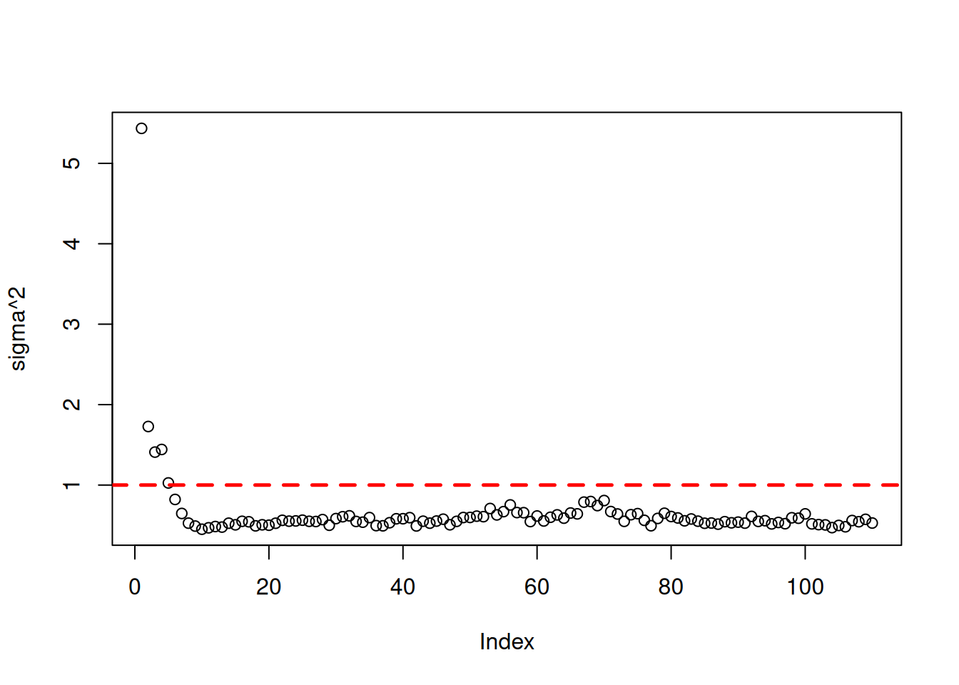

y_hat_test <- predict(bart_model, X=X_test, type="mean", terms="y_hat")
plot(y_hat_test, y_test, pch=16, cex=0.75, xlab = "pred", ylab = "actual")
abline(0,1,col="red",lty=2,lwd=2.5)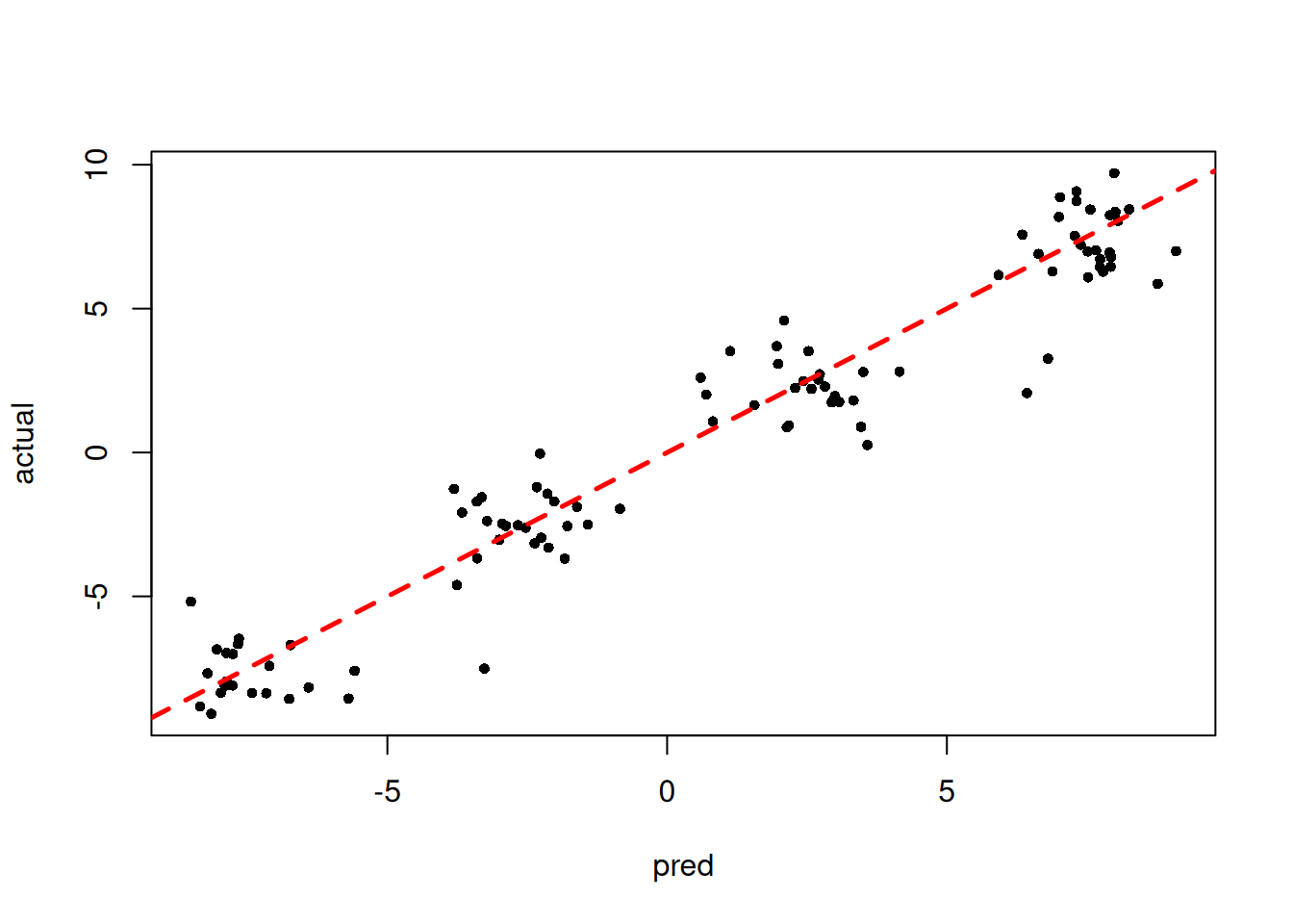

Python

fig, (ax1, ax2) = plt.subplots(1, 2, figsize=(12, 4))

sigma2_samples = bart_model.extract_parameter("sigma2_global")
ax1.plot(sigma2_samples)
ax1.axhline(noise_sd**2, color="red", linestyle="dashed", linewidth=2)
ax1.set_ylabel(r"$\sigma^2$")

y_hat_test = bart_model.predict(X=X_test, terms="y_hat", type="mean")
ax2.scatter(y_hat_test, y_test, s=15, alpha=0.6)
lo = min(y_hat_test.min(), y_test.min())
hi = max(y_hat_test.max(), y_test.max())
ax2.plot([lo, hi], [lo, hi], color="red", linestyle="dashed", linewidth=2)
ax2.set_xlabel("pred")
ax2.set_ylabel("actual")

plt.tight_layout()
plt.show()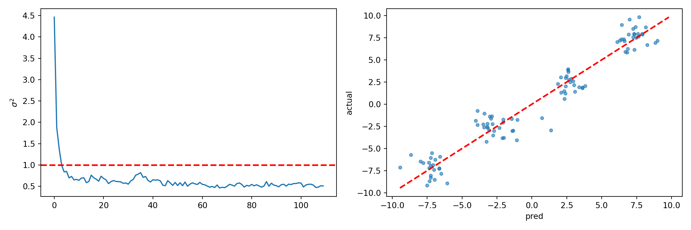

Variable Split Counts

The get_forest_split_counts method of a BART model’s internal forest objects allows us to compute the number of times each variable was used in a split rule across all trees in a given forest.

Below we query this vector for the final GFR sample (1-indexed as 10 in R, 0-indexed as 9 in Python), where the second argument is the dimensionality of the covariates.

R

bart_model$mean_forests$get_forest_split_counts(10, p_x)

 [1] 29 30 23 29 25 19 39 20 32 33

Python

bart_model.forest_container_mean.get_forest_split_counts(9, p_x)

array([22, 27, 18, 20, 25, 30, 21, 33, 27, 41], dtype=int32)

We can also compute split counts for each feature aggregated over all forests

R

bart_model$mean_forests$get_aggregate_split_counts(p_x)

 [1] 1971 2825 2382 2900 3009 2462 3431 2076 3226 3606

Python

bart_model.forest_container_mean.get_overall_split_counts(p_x)

array([2436, 2711, 2076, 2161, 2664, 2622, 2250, 3103, 2522, 4531],
      dtype=int32)

The split counts appear relatively uniform across features, so let’s dig deeper and look at individual trees.

The get_granular_split_counts method returns a 3-dimensional array of shape (num_forests, num_trees, num_features), where each entry represents the number of times a feature was used in a split for a specific tree in a specific forest.

That is, we can count the number of times feature \(k\) was split on in tree \(j\) of forest \(i\) by looking at the (i,j,k) entry of this array.

Below we compute the split count for all features in the first tree of the last GFR sample in our model (noting again the use of 1-indexing in R and 0-indexing in Python).

R

splits = bart_model$mean_forests$get_granular_split_counts(p_x)
splits[10,1,]

 [1] 0 0 0 0 0 0 0 0 0 1

Python

splits = bart_model.forest_container_mean.get_granular_split_counts(p_x)
splits[9, 0, :]

array([0, 0, 0, 0, 0, 0, 0, 0, 0, 1], dtype=int32)

This tree has a single split on the only “important” feature (10). Now, let’s look at the second tree.

R

splits[10,2,]

 [1] 0 0 0 0 0 0 0 0 0 2

Python

splits[9, 1, :]

array([0, 0, 0, 0, 0, 0, 0, 0, 0, 1], dtype=int32)

And the 20th and 30th trees

R

splits[10,20,]

 [1] 1 1 0 0 0 0 1 0 0 1

Python

splits[9, 19, :]

array([0, 0, 0, 0, 0, 0, 0, 1, 0, 0], dtype=int32)

R

splits[10,30,]

 [1] 0 0 0 1 0 0 0 0 0 0

Python

splits[9, 29, :]

array([0, 0, 0, 0, 0, 1, 0, 0, 0, 0], dtype=int32)

We see that “later” trees are splitting on other features, but we also note that these trees are fitting an outcome that is already residualized by many “relevant splits” made by trees 1 and 2.

Tree Structure

Now, let’s inspect the first tree for the last GFR sample in more depth, following this scikit-learn vignette.

R

forest_num <- 9
tree_num <- 0
nodes <- sort(bart_model$mean_forests$nodes(forest_num, tree_num))
for (nid in nodes) {
    if (bart_model$mean_forests$is_leaf_node(forest_num, tree_num, nid)) {
        node_depth <- bart_model$mean_forests$node_depth(forest_num, tree_num, nid)
        space_text <- rep("\t", node_depth)
        leaf_values <- bart_model$mean_forests$node_leaf_values(forest_num, tree_num, nid)
        cat(space_text, "node=", nid, " is a leaf node with value=",
            format(leaf_values, digits = 3), "\n", sep = "")
    } else {
        node_depth <- bart_model$mean_forests$node_depth(forest_num, tree_num, nid)
        space_text <- rep("\t", node_depth)
        left <- bart_model$mean_forests$left_child_node(forest_num, tree_num, nid)
        feature <- bart_model$mean_forests$node_split_index(forest_num, tree_num, nid)
        threshold <- bart_model$mean_forests$node_split_threshold(forest_num, tree_num, nid)
        right <- bart_model$mean_forests$right_child_node(forest_num, tree_num, nid)
        cat(space_text, "node=", nid, " is a split node, which tells us to go to node ",
            left, " if X[:, ", feature, "] <= ", format(threshold, digits = 3),
            " else to node ", right, "\n", sep = "")
    }
}

node=0 is a split node, which tells us to go to node 1 if X[:, 9] <= 0.508 else to node 2
    node=1 is a leaf node with value=-0.372
    node=2 is a leaf node with value=0.312

Python

forest_num = 9
tree_num = 0
fc = bart_model.forest_container_mean
nodes = np.sort(fc.nodes(forest_num, tree_num))
for nid in nodes:
    depth = fc.node_depth(forest_num, tree_num, nid)
    indent = "\t" * depth
    if fc.is_leaf_node(forest_num, tree_num, nid):
        value = np.round(fc.node_leaf_values(forest_num, tree_num, nid), 3)
        print(f"{indent}node={nid} is a leaf node with value={value}")
    else:

        left = fc.left_child_node(forest_num, tree_num, nid)
        feature = fc.node_split_index(forest_num, tree_num, nid)
        threshold = round(fc.node_split_threshold(forest_num, tree_num, nid), 3)
        right = fc.right_child_node(forest_num, tree_num, nid)
        print(f"{indent}node={nid} is a split node, which tells us to go to node "
              f"{left} if X[:, {feature}] <= {threshold} else to node {right}")

node=0 is a split node, which tells us to go to node 1 if X[:, 9] <= 0.488 else to node 2
    node=1 is a leaf node with value=[-0.272]
    node=2 is a leaf node with value=[0.324]