Probit BART for Binary Outcomes

This vignette demonstrates how to run BART / BCF on binary outcomes via the probit link in stochtree.

The original Chipman et al. (2010) BART paper describes this model for a binary outcome variable \(Y_i\) and covariate vector \(x_i\),

\[\begin{aligned} \Pr(Y_i = 1 \mid x_i) &\sim \Phi(f(x_i)),\\ f &\sim \mathrm{BART}(\alpha, \beta, m) \end{aligned}\]

where \(\Phi(\cdot)\) denotes the standard normal CDF.

We can sample from this model using the data augmentation of Albert and Chib (1993). Letting \(Z_i \sim N(f(x_i), 1)\) and \(Y_i = \mathcal{1}\left(Z_i > 0\right)\), we can sample \(Z_i\) via a truncated normal distribution in which observations with \(Y_i = 0\) are truncated above at 0 and observations with \(Y_i = 1\) are truncated below at 0.

Setup

Load necessary packages

R

library(stochtree)

Python

import numpy as np
import matplotlib.pyplot as plt
from stochtree import OutcomeModel
from stochtree import BARTModel

Set a random seed

R

random_seed = 1234
set.seed(random_seed)

Python

random_seed = 1234
rng = np.random.default_rng(random_seed)

Supervised Learning Demo

Here, we generate data from a probit model

\[\begin{aligned} X_1,\dots,X_p &\sim \text{U}\left(-1,1\right)\\ Z &= \eta_0 + 2 X_1 - X_2 + \epsilon\\ \epsilon &\sim \mathcal{N}\left(0,1\right)\\ Y &= \mathbb{1}\left(Z > 0\right) \end{aligned}\]

\(\eta_0\) controls the “class imbalance” of the data. With \(\eta_0 = 0\), \(Y = 1\) with roughly equal probability to 0. With \(\eta_0 < 0\), \(Y = 0\) with higher probability, and vice versa for \(\eta_0 > 0\). This is handled in stochtree via a fixed “offset” term so that a centered \(Z\) is sampled by the model.

Simulation

Generate data from the DGP above, with \(\eta_0 = -1\) for moderate class imbalance.

R

n <- 2000
p_x <- 5
X <- matrix(runif(n * p_x, min = -1, max = 1), ncol = p_x)
eta_0 <- -1
f_X <- eta_0 + 2 * X[, 1] - X[, 2]
Z <- f_X + rnorm(n, 0, 1)
y <- (Z > 0) * 1

Python

n, p_x = 2000, 5
X = rng.uniform(size=(n, p_x), low = -1, high = 1)
eta_0 = -1
f_X = eta_0 + 2 * X[:,0] - X[:,1]
Z = f_X + rng.standard_normal(size=(n,))
y = (Z > 0) * 1

We first check the class imbalance and see that there are about 3x as many 0s as 1s.

R

table(y)

y
   0    1 
1455  545 

Python

vals, counts = np.unique(y, return_counts=True)
for v, c in zip(vals, counts):
    print(f"{v}: {c}")

0: 1409
1: 591

Split into train and test sets

R

test_set_pct <- 0.2
n_test <- round(test_set_pct * n)
n_train <- n - n_test
test_inds <- sort(sample(1:n, n_test, replace = FALSE))
train_inds <- (1:n)[!((1:n) %in% test_inds)]
X_test <- as.data.frame(X[test_inds, ])
X_train <- as.data.frame(X[train_inds, ])
Z_test <- Z[test_inds]
Z_train <- Z[train_inds]
y_test <- y[test_inds]
y_train <- y[train_inds]
f_x_test <- f_X[test_inds]
f_x_train <- f_X[train_inds]

Python

test_set_pct = 0.2
n_test = round(test_set_pct * n)
test_inds = rng.choice(n, n_test, replace=False)
train_inds = np.setdiff1d(np.arange(n), test_inds)
X_test, X_train = X[test_inds], X[train_inds]
Z_test, Z_train = Z[test_inds], Z[train_inds]
y_test, y_train = y[test_inds], y[train_inds]
f_x_test, f_x_train = f_X[test_inds], f_X[train_inds]

Sampling and Analysis

We sample four chains from the probit model.

R

num_gfr <- 0
num_burnin <- 500
num_mcmc <- 1000
general_params <- list(
  sample_sigma2_global = F,
  num_chains = 4,
  num_threads = 1,
  random_seed = random_seed,
  outcome_model = OutcomeModel(outcome = "binary", link = "probit")
)
mean_forest_params <- list(sample_sigma2_leaf = F)
bart_model <- stochtree::bart(
  X_train = X_train,
  y_train = y_train,
  X_test = X_test,
  num_gfr = num_gfr,
  num_burnin = num_burnin,
  num_mcmc = num_mcmc,
  general_params = general_params,
  mean_forest_params = mean_forest_params
)

Python

num_gfr = 0
num_burnin = 500
num_mcmc = 1000
bart_model = BARTModel()
bart_model.sample(
    X_train=X_train,
    y_train=y_train,
    X_test=X_test,
    num_gfr=num_gfr,
    num_burnin=num_burnin,
    num_mcmc=num_mcmc,
    general_params={
        "sample_sigma2_global": False,
        "num_threads": 1,
        "num_chains": 4,
        "random_seed": random_seed,
        "outcome_model": OutcomeModel(outcome = "binary", link = "probit")
    },
    mean_forest_params={"sample_sigma2_leaf": False},
)

We inspect the model by plotting the true latent \(Z\) against their forest-based predictions

R

Z_hat_test <- predict(
  bart_model,
  X = X_test,
  terms = "mean_forest",
  type = "mean"
)
plot(
  Z_hat_test,
  Z_test,
  pch = 16,
  cex = 0.75,
  xlab = "Predicted",
  ylab = "Actual",
  main = "Latent outcome"
)
abline(0, 1, col = "red", lty = 2, lwd = 2.5)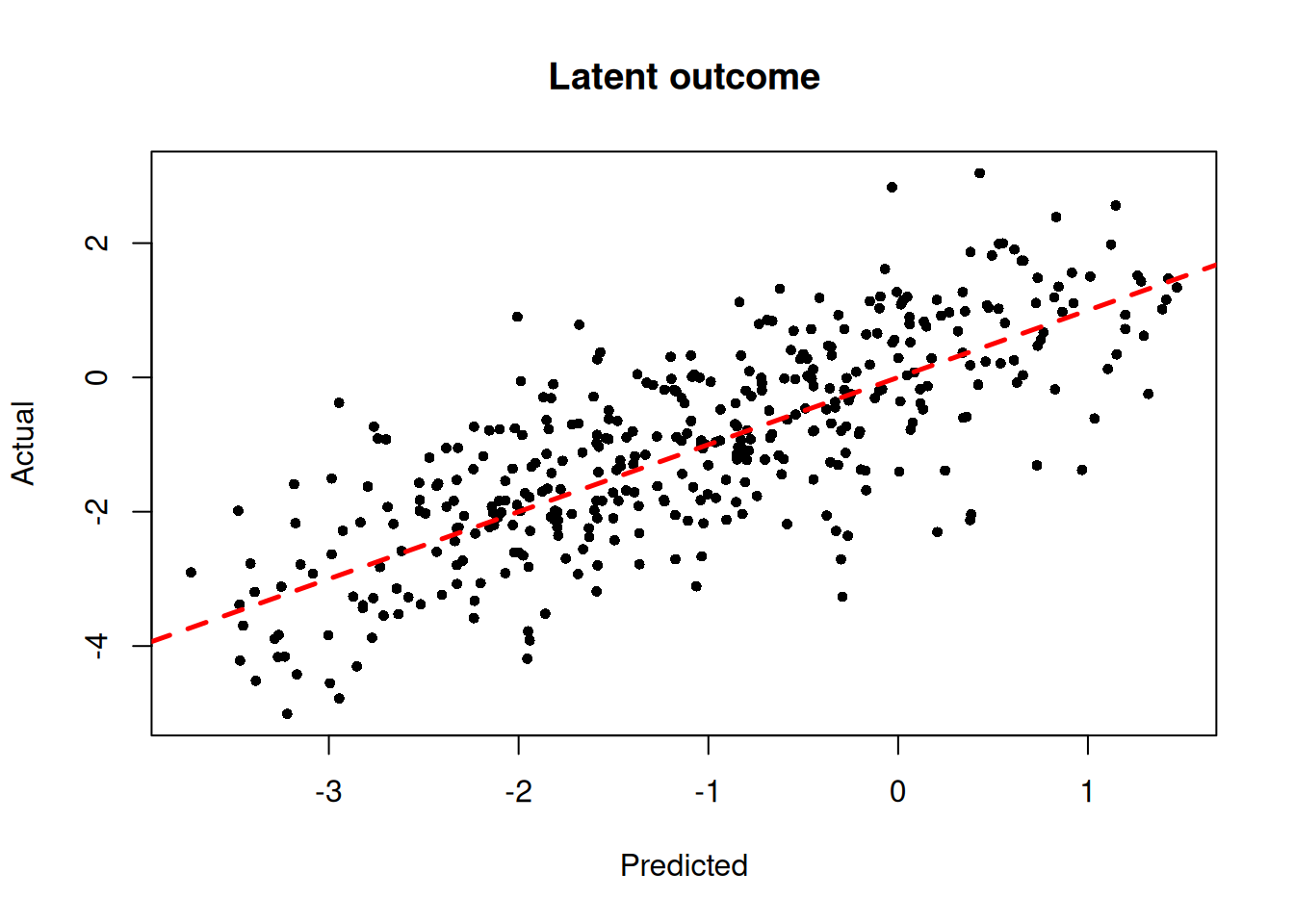

Python

Z_hat_test = bart_model.predict(X=X_test, terms="mean_forest", type="mean")
lo, hi = (
    min(Z_hat_test.min(), (Z_test).min()),
    max(Z_hat_test.max(), (Z_test).max()),
)
plt.scatter(Z_hat_test, Z_test, s=10, alpha=0.6)
plt.plot([lo, hi], [lo, hi], color="red", linestyle="dashed", linewidth=2)
plt.xlabel("Predicted")
plt.ylabel("Actual")
plt.title("Latent outcome")
plt.show()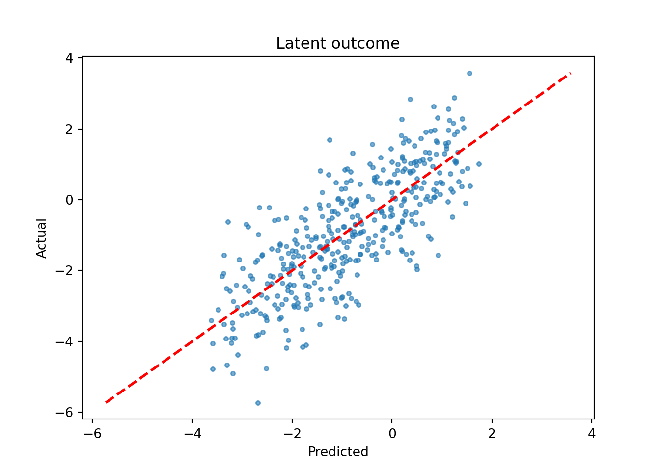

References

Albert, James H, and Siddhartha Chib. 1993. “Bayesian Analysis of Binary and Polychotomous Response Data.” Journal of the American Statistical Association 88 (422): 669–79.

Chipman, Hugh A., Edward I. George, and Robert E. McCulloch. 2010. “BART: Bayesian additive regression trees.” The Annals of Applied Statistics 4 (1): 266–98. https://doi.org/10.1214/09-AOAS285.