Model Prediction and Parameter Extraction

Introduction

The vignettes in the Core Models section demonstrate how to fit different types of models in stochtree. This vignette walks through the interfaces for querying and extracting parameters from fitted stochtree models.

There are two primary interfaces for interacting with trained BART / BCF models:

1. Prediction: obtaining estimates for model terms that depend on covariates or other input data
   • In R, this is governed by an overloaded predict() function that specializes to BART and BCF so that predict(bart_model, ...) and predict(bcf_model, ...) return the requested predictions from the provided model
   • In Python, the BARTModel and BCFModel classes define predict() methods that can be called directly to obtain model predictions
2. Parameter Extraction: obtaining samples / traces of parametric model terms (such as the global error scale, \(\sigma^2\))
   • In R, this is governed by an overloaded extractParameter() function that specializes to BART and BCF so that extractParameter(bart_model, ...) and extractParameter(bcf_model, ...) return the requested samples from the provided model
   • In Python, the BARTModel and BCFModel classes define extract_parameter() methods that can be called directly to obtain parameter estimates

Prediction

The prediction interface is designed to be as flexible as the class of models that stochtree supports. The broad pattern that input data is provided for a given model and the corresponding predict method returns predictions for one or more model terms, with some optional user-requested transformations.

BART

The BART Prediction API differs stylistically in R and Python but provides the same functionality, which we annotate below

R

predict(
  object,
  X,
  leaf_basis = NULL,
  rfx_group_ids = NULL,
  rfx_basis = NULL,
  type = "posterior",
  terms = "all",
  scale = "linear"
)

1

Reference to the sampled BART model

2

Covariates: all BART models require covariates so these are not optional in the predict method

3

Leaf basis: required if the original model was fit with a leaf basis

4

Random effects group labels: required if the original model was fit with an additive random effects term

5

Random effects basis: required if the original model was fit with an additive random effects term with custom basis (i.e. model_spec was not "intercept_only")

6

Whether predictions should return each posterior draw ('posterior') or be averaged across the posterior ('mean')

7

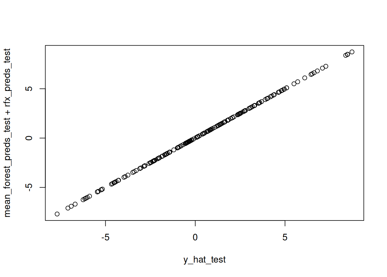
Which model terms to return predictions for. 'all' returns every model term available, 'y_hat' returns only outcome predictions, 'mean_forest' returns mean forest predictions (if available), 'rfx' returns random effects predictions (if available), and 'variance_forest' returns variance forest predictions (if available)

8

Whether predictions should be returned as-is from forest / RFX terms (scale = 'linear'), transformed to probabilities (scale = 'probability') or class labels (scale = 'class')

Python

bart.BARTModel.predict(
  X,
  leaf_basis=None,
  rfx_group_ids=None,
  rfx_basis=None,
  type='posterior',
  terms='all',
  scale='linear',
)

1

.predict() called from a reference to the sampled BART model

2

Covariates: all BART models require covariates so these are not optional in the predict method

3

Leaf basis: required if the original model was fit with a leaf basis

4

Random effects group labels: required if the original model was fit with an additive random effects term

5

Random effects basis: required if the original model was fit with an additive random effects term with custom basis (i.e. model_spec was not "intercept_only")

6

Whether predictions should return each posterior draw ('posterior') or be averaged across the posterior ('mean')

7

Which model terms to return predictions for. 'all' returns every model term available, 'y_hat' returns only outcome predictions, 'mean_forest' returns mean forest predictions (if available), 'rfx' returns random effects predictions (if available), and 'variance_forest' returns variance forest predictions (if available)

8

Whether predictions should be returned as-is from forest / RFX terms (scale = 'linear'), transformed to probabilities (scale = 'probability') or class labels (scale = 'class')

The data inputs to this API are fairly straightforward, but the type, terms and scale arguments merit some detailed (language-agnostic) explanation.

The BART overview page has a more in-depth review of the BART model, but the most complex version a BART model that stochtree supports is, mathematically, \[ \begin{aligned} y_{i,j} \mid \Psi_{i,j} = \psi_{i,j}, X_{i,j} = x_{i,j}, W_{i,j} = w_{i,j} &\sim \mathcal{N}\left(w_{i,j} \vec{\gamma}_j + f(x_{i,j}, \psi_{i,j}), \sigma^2_0 \exp{h(x_{i,j})}\right),\\ f &\sim \text{BART}(\alpha_f, \beta_f, m_f), \\ h &\sim \text{logBART}(\alpha_h, \beta_h, m_h), \\ \vec{\gamma}_j &\sim \mathrm{N}(\vec{0}, \sigma^2_{\gamma} I). \end{aligned} \]

This model has:

1. Linear leaf regression on a basis \(\Psi\)
2. Forest-based heteroskedasticity, defined by a \(\text{logBART}\) prior on \(h\)
3. Additive random effects on basis \(W\)

Prediction Terms

Each of the individual options for the terms argument can be mapped to the equation above:

Term	Mathematical Representation
y_hat	\(w_{i,j} \vec{\gamma}_j + f(x_{i,j}, \psi_{i,j})\)
mean_forest	\(f(x_{i,j}, \psi_{i,j})\)
rfx	\(w_{i,j} \vec{\gamma}_j\)
variance_forest	\(\sigma^2_0 \exp{h(x_{i,j})}\)

Requesting terms = 'all' will yield a list / dictionary with each of the terms above stored as separate entries. For models without a variance forest, terms = 'variance_forest' will be ignored. For models without random effects, terms = 'rfx' will be ignored and y_hat collapses to \(f(x_{i}, \psi_{i})\). For models without leaf regression, mean_forest and y_hat collapse to \(f(x_i)\).

Prediction Type

If a BART model has been sampled for \(mc\) iterations, then most of the above terms will be \(n \times mc\) matrices, where \(n\) is the number of rows in X, representing a posterior distribution over \(f\), \(h\) or the conditional outcome mean. This can be converted to a “simple” \(n\)-dimensional posterior mean (useful for prediction when terms = 'y_hat', for example) by averaging over the \(mc\) columns. This use case is common enough that stochtree will perform the aggregation before returning to users if type = 'mean' is specified.

Prediction Scale

In addition to the Gaussian model for continuous outcomes in the equation above, stochtree supports modeling binary outcomes through a probit link and ordinal outcomes through a cloglog link. Both of these models apply transformations to model discrete outcomes with continuous forest predictions, and the scale argument lets users determine which transformation (if any) to apply to model predictions.

Probit

The probit model precludes a variance forest, but works with both random effects and leaf regression. Specifying scale = 'linear' returns predictions as returned by the mean forest and random effects terms, scale = 'probability' converts the predictions into that term’s contribution to the conditional probability of y = 1, and scale = 'class' returns the category index with the highest predicted probability.

Term	scale = 'linear'	scale = 'probability'
y_hat	\(w_{i,j} \vec{\gamma}_j + f(x_{i,j}, \psi_{i,j})\)	\(\Phi\left(w_{i,j} \vec{\gamma}_j + f(x_{i,j}, \psi_{i,j})\right)\)
mean_forest	\(f(x_{i,j}, \psi_{i,j})\)	\(\Phi\left(f(x_{i,j}, \psi_{i,j})\right)\)
rfx	\(w_{i,j} \vec{\gamma}_j\)	\(\Phi\left(w_{i,j} \vec{\gamma}_j\right)\)

where \(\Phi(\cdot)\) is the standard normal CDF.

Cloglog

The cloglog model precludes a variance forest, random effects, or leaf regression. Specifying scale = 'linear' returns predictions as returned by the mean forest, scale = 'probability' converts the predictions into the conditional probability of each outcome category, and scale = 'class' returns the category index with the highest predicted probability.

Term	scale = 'linear'	scale = 'probability'
y_hat	\(f(x_{i})\)	\(\exp(-\exp(c_{k-1}+f(x_i))) - \exp(-\exp(c_{k}+f(x_i)))\)
mean_forest	\(f(x_{i})\)	\(\exp(-\exp(c_{k-1}+f(x_i))) - \exp(-\exp(c_{k}+f(x_i)))\)

Note that \(k\) denotes a category index and \(c_k\) is a category-specific “cutpoint” parameter unique to the cloglog model.

BCF

The multilingual BCF Prediction API is annotated below as with the BART API

R

predict(
  object,
  X,
  Z,
  propensity = NULL,
  rfx_group_ids = NULL,
  rfx_basis = NULL,
  type = "posterior",
  terms = "all",
  scale = "linear"
)

1

Reference to the sampled BCF model

2

Covariates: all BCF models require covariates so these are not optional in the predict method

3

Treatment: all BCF models require treatment so this is not optional in the predict method

4

Propensity: required if the original model was fit with a user-supplied propensity score

5

Random effects group labels: required if the original model was fit with an additive random effects term

6

Random effects basis: required if the original model was fit with an additive random effects term with custom basis (i.e. model_spec was not "intercept_only")

7

Whether predictions should return each posterior draw ('posterior') or be averaged across the posterior ('mean')

8

Which model terms to return predictions for. 'all' returns every model term available, 'y_hat' returns only outcome predictions, 'mu' returns prognostic forest predictions, 'tau' returns treatment effect forest predictions (and \(\tau_0\) intercept, if available), 'prognostic_forest' returns prognostic forest predictions and any random intercepts modeled by a random effects model_spec of 'intercept_only' or 'intercept_plus_treatment', 'cate' returns treatment effect forest predictions and any random treatment effect modeled by a random effects model_spec of 'intercept_plus_treatment', 'rfx' returns random effects predictions (if available), and 'variance_forest' returns variance forest predictions (if available)

9

Whether predictions should be returned as-is from forest / RFX terms (scale = 'linear'), transformed to probabilities (scale = 'probability') or class labels (scale = 'class')

Python

bcf.BCFModel.predict(
  X,
  Z,
  propensity=None,
  rfx_group_ids=None,
  rfx_basis=None,
  type='posterior',
  terms='all',
  scale='linear',
)

1

.predict() called from a reference to the sampled BART model

2

Covariates: all BCF models require covariates so these are not optional in the predict method

3

Treatment: all BCF models require treatment so this is not optional in the predict method

4

Propensity: required if the original model was fit with a user-supplied propensity score

5

Random effects group labels: required if the original model was fit with an additive random effects term

6

Random effects basis: required if the original model was fit with an additive random effects term with custom basis (i.e. model_spec was not "intercept_only")

7

Whether predictions should return each posterior draw ('posterior') or be averaged across the posterior ('mean')

8

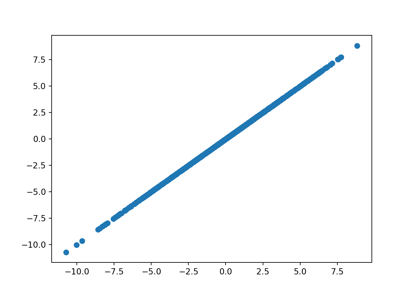
Which model terms to return predictions for. 'all' returns every model term available, 'y_hat' returns only outcome predictions, 'mu' returns prognostic forest predictions, 'tau' returns treatment effect forest predictions (and \(\tau_0\) intercept, if available), 'prognostic_forest' returns prognostic forest predictions and any random intercepts modeled by a random effects model_spec of 'intercept_only' or 'intercept_plus_treatment', 'cate' returns treatment effect forest predictions and any random treatment effect modeled by a random effects model_spec of 'intercept_plus_treatment', 'rfx' returns random effects predictions (if available), and 'variance_forest' returns variance forest predictions (if available)

9

Whether predictions should be returned as-is from forest / RFX terms (scale = 'linear'), transformed to probabilities (scale = 'probability') or class labels (scale = 'class')

The data inputs to this API are fairly straightforward, but the type, terms and scale arguments merit some detailed (language-agnostic) explanation.

The BCF overview page has a more in-depth review of the BCF model, but the most complex version a BCF model that stochtree supports is, mathematically, \[ \begin{aligned} y_{i,j} \mid - &\sim \mathcal{N}\left(\gamma_{0,j} + f_0(x_{i,j}) + \gamma_{1,j} z_{i,j} + \left(b_1 z_{i,j} + b_0 (1-z_{i,j}) \right) \left[\tau_0 + t(x_{i,j})\right], \sigma^2_0 \exp{h(x_{i,j})}\right),\\ f_0 &\sim \text{BART}(\alpha_0, \beta_0, m_0), \\ t &\sim \text{BART}(\alpha_t, \beta_t, m_t), \\ h &\sim \text{logBART}(\alpha_h, \beta_h, m_h), \\ \tau_0 &\sim \mathcal{N}(0, \sigma^2_{\tau}), \\ b_0, b_1 &\sim \mathcal{N}(0, 1/2), \\ \gamma_{0,j}, \gamma_{1,j} &\sim \mathrm{N}(0, \sigma^2_{\gamma}). \end{aligned} \]

This model has:

1. Binary treatment with adaptive coding
2. Treatment effect function decomposed into parametric (\(\tau_0\)) and nonparametric (\(t(X)\)) terms (i.e. the sample_intercept option in the treatment_effect_forest_params list / dictionary)
3. Forest-based heteroskedasticity
4. Additive random effects on the intercept_plus_treatment basis of \([1,Z]\)

Prediction Terms

Each of the individual options for the terms argument can be mapped to the equation above:

Term	Mathematical Representation
y_hat	\(\gamma_{0,j} + f_0(x_{i,j}) + \gamma_{1,j} z_{i,j} + \left(b_1 z_{i,j} + b_0 (1-z_{i,j}) \right) \left[\tau_0 + t(x_{i,j})\right]\)
mu	\(f_0(x_{i,j}) + b_0 \left[\tau_0 + t(x_{i,j})\right]\)
prognostic_function	\(\gamma_{0,j} + f_0(x_{i,j}) + b_0 \left[\tau_0 + t(x_{i,j})\right]\)
tau	\(\left( b_1 - b_0 \right) \left[\tau_0 + t(x_{i,j})\right]\)
cate	\(\gamma_{1,j} + \left( b_1 - b_0 \right) \left[\tau_0 + t(x_{i,j})\right]\)
rfx	\(\gamma_{0,j} + \gamma_{1,j} z_{i,j}\)
variance_forest	\(\sigma^2_0 \exp{h(x_{i,j})}\)

Requesting terms = 'all' will yield a list / dictionary with each of the terms above stored as separate entries. For models without a variance forest, terms = 'variance_forest' will be ignored. For models without random effects, terms = 'rfx' will be ignored and y_hat collapses to \(f_0(x_{i,j}) + \left(b_1 z_{i,j} + b_0 (1-z_{i,j}) \right) \left[\tau_0 + t(x_{i,j})\right]\), and both 'mu' and 'prognostic_function' as well as 'tau' and 'cate' will be the same.

Without adaptive coding, the terms simplify to

Term	Mathematical Representation
y_hat	\(\gamma_{0,j} + f_0(x_{i,j}) + z_{i,j} \left[\gamma_{1,j} + \tau_0 + t(x_{i,j})\right]\)
mu	\(f_0(x_{i,j})\)
prognostic_function	\(\gamma_{0,j} + f_0(x_{i,j})\)
tau	\(\tau_0 + t(x_{i,j})\)
cate	\(\gamma_{1,j} + \tau_0 + t(x_{i,j})\)
rfx	\(\gamma_{0,j} + \gamma_{1,j} z_{i,j}\)
variance_forest	\(\sigma^2_0 \exp{h(x_{i,j})}\)

Similarly, without a parametric treatment effect, the terms simplify to

Term	Mathematical Representation
y_hat	\(\gamma_{0,j} + f_0(x_{i,j}) + \gamma_{1,j} z_{i,j} + \left(b_1 z_{i,j} + b_0 (1-z_{i,j}) \right) t(x_{i,j})\)
mu	\(f_0(x_{i,j}) + b_0 t(x_{i,j})\)
prognostic_function	\(\gamma_{0,j} + f_0(x_{i,j}) + b_0 t(x_{i,j})\)
tau	\(\left( b_1 - b_0 \right) t(x_{i,j})\)
cate	\(\gamma_{1,j} + \left( b_1 - b_0 \right) t(x_{i,j})\)
rfx	\(\gamma_{0,j} + \gamma_{1,j} z_{i,j}\)
variance_forest	\(\sigma^2_0 \exp{h(x_{i,j})}\)

Prediction Type

As with BART, stochtree will average over posterior samples before returning to users if type = 'mean' is specified.

Prediction Scale

In addition to the Gaussian model for continuous outcomes in the equation above, stochtree supports modeling binary outcomes through a probit link, and the scale argument lets users determine which transformation (if any) to apply to model predictions.

The probit model precludes a variance forest, but works with random effects and most other BCF modeling features. Specifying scale = 'linear' returns predictions as returned by the mean forest and random effects terms, scale = 'probability' converts the predictions into that term’s contribution to the conditional probability of y = 1, and scale = 'class' returns the category index with the highest predicted probability.

Parameter Extraction

Most BART and BCF models include one or more parametric terms, stored internally as vectors / arrays. Similarly, BART and BCF models often cache predictions for forest terms internally during sampling. stochtree provides a standard API for extracting these samples from fitted BART / BCF models.

BART

The BART parameter extraction API differs stylistically in R and Python but provides the same functionality, which we annotate below

R

extractParameter(
  object,
  term,
)

1

Reference to the sampled BART model

2

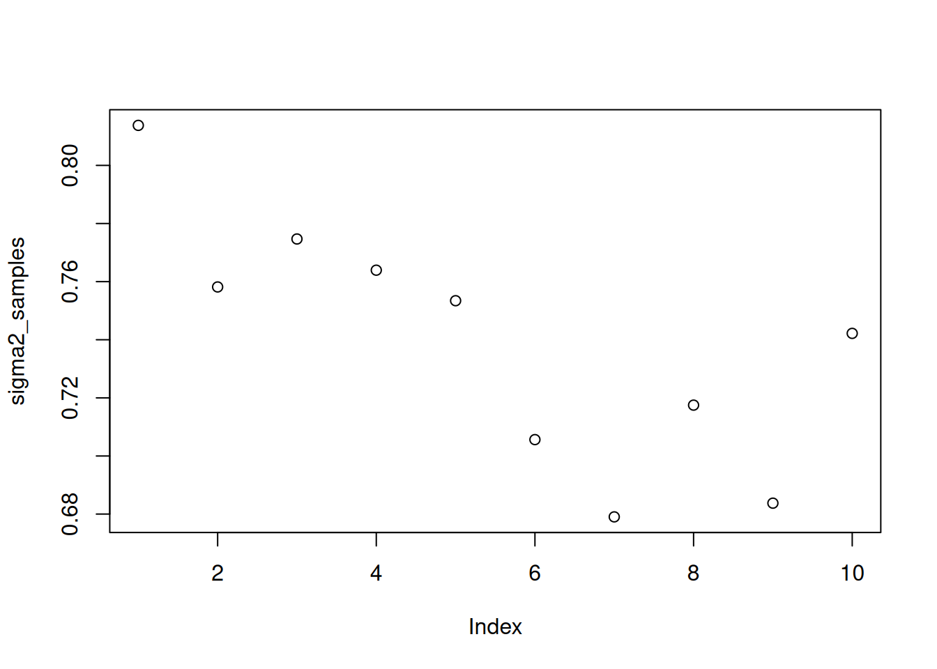
Which internal model samples to extract. Options include "sigma2", "global_error_scale", "sigma2_global", "sigma2_leaf", "leaf_scale", "y_hat_train", "y_hat_test", "sigma2_x_train", "var_x_train", "sigma2_x_test", "var_x_test", "cloglog_cutpoints", "cutpoints"

Python

bart.BARTModel.extract_parameter(
  term,
)

1

.extract_parameter() called from a reference to the sampled BART model

2

Which internal model samples to extract. Options include "sigma2", "global_error_scale", "sigma2_global", "sigma2_leaf", "leaf_scale", "y_hat_train", "y_hat_test", "sigma2_x_train", "var_x_train", "sigma2_x_test", "var_x_test", "cloglog_cutpoints", "cutpoints"

This method extracts a vector, matrix, or array of samples from a BART model, queried by name. Random effects are handled by a separate extract_parameter_samples method attached to the underlying RandomEffectsContainer object due to the complexity of the random effects parameters. If the requested model term is not found, an error is thrown. The following conventions are used for parameter names:

1. Global error variance: "sigma2", "global_error_scale", "sigma2_global"
2. Leaf scale: "sigma2_leaf", "leaf_scale"
3. In-sample mean function predictions: "y_hat_train"
4. Test set mean function predictions: "y_hat_test"
5. In-sample variance forest predictions: "sigma2_x_train", "var_x_train"
6. Test set variance forest predictions: "sigma2_x_test", "var_x_test"
7. Ordinal model cutpoints (valid only for ordinal cloglog models): "cloglog_cutpoints", "cutpoints"

BCF

The multilingual BCF parameter extraction API is annotated below as with the BART API

R

extractParameter(
  object,
  term,
)

1

Reference to the sampled BCF model

2

Which internal model samples to extract. Options include "sigma2", "global_error_scale", "sigma2_global", "sigma2_leaf_mu", "leaf_scale_mu", "mu_leaf_scale", "sigma2_leaf_tau", "leaf_scale_tau", "tau_leaf_scale", "adaptive_coding", "y_hat_train", "y_hat_test", "tau_hat_train", "tau_hat_test", "tau_0", "treatment_intercept", "tau_intercept", "sigma2_x_train", "var_x_train", "sigma2_x_test", "var_x_test"

Python

bcf.BCFModel.extract_parameter(
  term,
)

1

.extract_parameter() called from a reference to the sampled BCF model

2

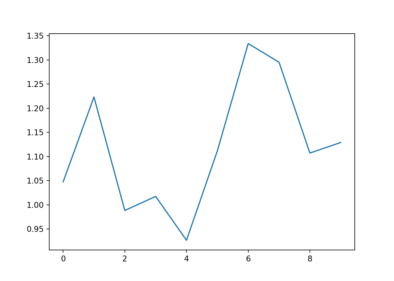
Which internal model samples to extract. Options include "sigma2", "global_error_scale", "sigma2_global", "sigma2_leaf_mu", "leaf_scale_mu", "mu_leaf_scale", "sigma2_leaf_tau", "leaf_scale_tau", "tau_leaf_scale", "adaptive_coding", "y_hat_train", "y_hat_test", "tau_hat_train", "tau_hat_test", "tau_0", "treatment_intercept", "tau_intercept", "sigma2_x_train", "var_x_train", "sigma2_x_test", "var_x_test"

This method extracts a vector, matrix, or array of samples from a BART model, queried by name. Random effects are handled by a separate extract_parameter_samples method attached to the underlying RandomEffectsContainer object due to the complexity of the random effects parameters. If the requested model term is not found, an error is thrown. The following conventions are used for parameter names:

1. Global error variance: "sigma2", "global_error_scale", "sigma2_global"
2. Prognostic forest leaf scale: "sigma2_leaf_mu", "leaf_scale_mu", "mu_leaf_scale"
3. Treatment effect forest leaf scale: "sigma2_leaf_tau", "leaf_scale_tau", "tau_leaf_scale"
4. Adaptive coding parameters: "adaptive_coding" (returns both the control and treated parameters jointly, with control in the first row and treated in the second row)
5. In-sample mean function predictions: "y_hat_train"
6. Test set mean function predictions: "y_hat_test"
7. In-sample treatment effect forest predictions: "tau_hat_train"
8. Test set treatment effect forest predictions: "tau_hat_test"
9. Treatment effect intercept: "tau_0", "treatment_intercept", "tau_intercept"
10. In-sample variance forest predictions: "sigma2_x_train", "var_x_train"
11. Test set variance forest predictions: "sigma2_x_test", "var_x_test"

Demos

We now illustrate these APIs with a series of demos. We start by loading the necessary packages.

R

library(stochtree)

Python

import numpy as np
import matplotlib.pyplot as plt
from sklearn.model_selection import train_test_split
from stochtree import BARTModel, BCFModel

Set a seed for reproducibility

R

random_seed = 1234
set.seed(random_seed)

Python

random_seed = 1234
rng = np.random.default_rng(random_seed)

Supervised Learning

We begin with a demo of the supervised learning (BART) use case. We simulate from a regression dataset with leaf-wise basis and group random effects.

R

n <- 1000
p_x <- 10
p_w <- 1
X <- matrix(runif(n * p_x), ncol = p_x)
W <- matrix(runif(n * p_w), ncol = p_w)
f_XW <- (((0 <= X[, 10]) & (0.25 > X[, 10])) *
  (-7.5 * W[, 1]) +
  ((0.25 <= X[, 10]) & (0.5 > X[, 10])) * (-2.5 * W[, 1]) +
  ((0.5 <= X[, 10]) & (0.75 > X[, 10])) * (2.5 * W[, 1]) +
  ((0.75 <= X[, 10]) & (1 > X[, 10])) * (7.5 * W[, 1]))
rfx_group_ids <- sample(1:3, n, replace = T)
rfx_params <- c(-2, 0, 2)
rfx_basis <- runif(n, -1, 1)
f_rfx <- rfx_params[rfx_group_ids] * rfx_basis
noise_sd <- 1
y <- f_XW + f_rfx + rnorm(n, 0, 1) * noise_sd

Python

n = 1000
p_x = 10
p_w = 1
X = rng.uniform(size=(n, p_x))
W = rng.uniform(size=(n, p_w))
f_XW = (
    ((X[:, 9] >= 0)    & (X[:, 9] < 0.25)) * (-7.5 * W[:, 0]) +
    ((X[:, 9] >= 0.25) & (X[:, 9] < 0.5))  * (-2.5 * W[:, 0]) +
    ((X[:, 9] >= 0.5)  & (X[:, 9] < 0.75)) * ( 2.5 * W[:, 0]) +
    ((X[:, 9] >= 0.75) & (X[:, 9] < 1.0))  * ( 7.5 * W[:, 0])
)
rfx_group_ids = rng.choice([0,1,2], size=(n,))
rfx_params = np.array([-2,0,2])
rfx_basis = rng.uniform(low=-1,high=1,size=(n,))
f_rfx = rfx_params[rfx_group_ids] * rfx_basis
y = f_XW + f_rfx + rng.standard_normal(n)

And we split the data into train and test sets

R

n_test <- 200
test_inds <- sample(1:n, n_test, replace = T)
train_inds <- (1:n)[!(1:n %in% test_inds)]
X_train <- X[train_inds, ]
X_test <- X[test_inds, ]
W_train <- W[train_inds, ]
W_test <- W[test_inds, ]
y_train <- y[train_inds]
y_test <- y[test_inds]
rfx_group_ids_train <- rfx_group_ids[train_inds]
rfx_group_ids_test <- rfx_group_ids[test_inds]
rfx_basis_train <- as.matrix(rfx_basis[train_inds])
rfx_basis_test <- as.matrix(rfx_basis[test_inds])

Python

n_test = 200
train_inds, test_inds = train_test_split(np.arange(n), train_size=n_test / n)
X_train, X_test = X[train_inds,:], X[test_inds,:]
W_train, W_test = W[train_inds,:], W[test_inds,:]
y_train, y_test = y[train_inds], y[test_inds]
rfx_group_ids_train, rfx_group_ids_test = rfx_group_ids[train_inds], rfx_group_ids[test_inds]
rfx_basis_train, rfx_basis_test = rfx_basis[train_inds], rfx_basis[test_inds]

Example 1(a): BART model without Random Effects or Leaf Regression

First, we fit a simple BART model without additive random effects or leaf regression.

R

num_gfr <- 5
num_burnin <- 0
num_mcmc <- 10
bart_model <- stochtree::bart(
  X_train = X_train,
  y_train = y_train,
  num_gfr = num_gfr,
  num_burnin = num_burnin,
  num_mcmc = num_mcmc
)

Python

num_gfr=5
num_burnin=0
num_mcmc=10
bart_model = BARTModel()
bart_model.sample(
    X_train=X_train,
    y_train=y_train,
    num_gfr=num_gfr,
    num_burnin=num_burnin,
    num_mcmc=num_mcmc,
)

We extract mean forest predictions and y_hat predictions and check that they agree

R

mean_forest_preds_test <- predict(
  bart_model,
  X = X_test,
  terms = "mean_forest",
  type = "mean"
)
y_hat_test <- predict(bart_model, X = X_test, terms = "y_hat", type = "mean")
plot(y_hat_test, mean_forest_preds_test)

Python

mean_forest_preds_test = bart_model.predict(X = X_test, terms = "mean_forest", type = "mean")
y_hat_test = bart_model.predict(X = X_test, terms = "y_hat", type = "mean")
plt.scatter(mean_forest_preds_test, y_hat_test)

We now extract and plot global error variance (\(\sigma^2\)) samples

R

sigma2_samples <- extractParameter(bart_model, term = "sigma2")
plot(sigma2_samples)

Python

sigma2_samples = bart_model.extract_parameter(term = "sigma2")
plt.plot(sigma2_samples)

Example 1(b): BART model with Random Effects and Leaf Regression

First, we fit a more complex BART model with additive random effects and leaf regression.

R

num_gfr <- 5
num_burnin <- 0
num_mcmc <- 10
bart_model <- stochtree::bart(
  X_train = X_train,
  leaf_basis_train = W_train,
  y_train = y_train,
  rfx_group_ids_train = rfx_group_ids_train,
  rfx_basis_train = rfx_basis_train,
  num_gfr = num_gfr,
  num_burnin = num_burnin,
  num_mcmc = num_mcmc
)

Python

num_gfr=5
num_burnin=0
num_mcmc=10
bart_model = BARTModel()
bart_model.sample(
    X_train=X_train,
    leaf_basis_train=W_train,
    y_train=y_train,
    rfx_group_ids_train=rfx_group_ids_train,
    rfx_basis_train=rfx_basis_train,
    num_gfr=num_gfr,
    num_burnin=num_burnin,
    num_mcmc=num_mcmc,
)

We extract mean forest predictions, RFX predictions and y_hat predictions and check that they can be combined to agree

R

mean_forest_preds_test <- predict(
  bart_model,
  X = X_test,
  leaf_basis = W_test,
  rfx_group_ids = rfx_group_ids_test,
  rfx_basis = rfx_basis_test,
  terms = "mean_forest",
  type = "mean"
)
rfx_preds_test <- predict(
  bart_model,
  X = X_test,
  leaf_basis = W_test,
  rfx_group_ids = rfx_group_ids_test,
  rfx_basis = rfx_basis_test,
  terms = "rfx",
  type = "mean"
)
y_hat_test <- predict(
  bart_model,
  X = X_test,
  leaf_basis = W_test,
  rfx_group_ids = rfx_group_ids_test,
  rfx_basis = rfx_basis_test,
  terms = "y_hat",
  type = "mean"
)
plot(y_hat_test, mean_forest_preds_test + rfx_preds_test)

Python

mean_forest_preds_test = bart_model.predict(
    X=X_test,
    leaf_basis=W_test,
    rfx_group_ids=rfx_group_ids_test,
    rfx_basis=rfx_basis_test,
    terms="mean_forest",
    type="mean",
)
rfx_preds_test = bart_model.predict(
    X=X_test,
    leaf_basis=W_test,
    rfx_group_ids=rfx_group_ids_test,
    rfx_basis=rfx_basis_test,
    terms="rfx",
    type="mean",
)
y_hat_test = bart_model.predict(
    X=X_test,
    leaf_basis=W_test,
    rfx_group_ids=rfx_group_ids_test,
    rfx_basis=rfx_basis_test,
    terms="y_hat",
    type="mean",
)
plt.scatter(mean_forest_preds_test + rfx_preds_test, y_hat_test)

We now extract and plot global error variance (\(\sigma^2\)) samples

R

sigma2_samples <- extractParameter(bart_model, term = "sigma2")
plot(sigma2_samples)

Python

sigma2_samples = bart_model.extract_parameter(term = "sigma2")
plt.plot(sigma2_samples)